ECONOMETRIC SPECIFICATION AND DATA
Given the conflicting results in the theoretical and empirical literature surveyed above, we now present our econometric framework for investigating the relationship between democracy, redistribution, and inequality.
We attempt to evaluate the diverse results within a single empirical strategy and sample, and we provide what we view to be some basic robust facts.In this section, we describe our econometric specifications and our main data. Our approach is to estimate a canonical panel data model with country fixed effects and time effects while also modeling the dynamics of inequality and redistribution. Both fixed effects and allowing for dynamics (e.g., mean reversion) are important. Without fixed effects, as already noted above, several confounding factors will make the association between democracy and inequality (or redistribution) difficult to interpret. Moreover, we will see that there are potentially important dynamics in the key outcome variables, and failure to control for this would lead to spurious relationships (or make it difficult to establish robust patterns even when such patterns do exist).
Some of the papers we mentioned above have adopted a set-up similar to this, for example Rodrik (1999), Ross (2006), Scheve and Stasavage (2009), Aghion et al. (2012), and Aidt andJensen (2013), but without modeling the dynamics in inequality or redistribution. In addition, several of these papers suffer from the “bad control” problem; for example, Scheve and Stasavage (2009) control for both suffrage and education in their investigation of the determinants of the top income shares. If democracy influences inequality via its impact on education, then such an empirical model is bound to find that democracy is not correlated with inequality. Even the pioneering paper by Aidt and Jensen (2013) controls for many endogenous variables on the right side of the regression including the Polity score of the country.[377]
21.4.1 EconometricSpecification
Consider the following simple econometric model:

where zit is the outcome of interest, which will be either (log of) tax revenue as a percentage of GDP or total revenue as a percentage of GDP as alternative measures of taxation, education, structural change, or one of several possible measures of inequality.
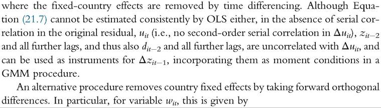
The dependent variables with significant skewness in their cross-country distribution, in particular, tax to GDP ratio, total government revenues to GDP ratio, agricultural shares of employment, and income and secondary enrollment, will be in logs, which makes interpretation easier and allows the impact of democracy to be proportional to the baseline level. All of the results emphasized in this paper also hold in specifications using levels rather than logs, but these are not reported to conserve space. Lags in this specification will always mean 5-year lags: dit~1 is democracy 5 years ago. The lagged value of the dependent variable on the right-hand side is included to capture persistence (and mean reversion) in these outcome measures, which may be a determinant of democracy or correlated with other variables that predict democracy. The main right hand side variable is dit, a dummy for democracy in country i in period t whose construction will be described in detail below. This variable is lagged by one period (generally a 5-year interval) because we expect its impact not to be contemporaneous. All other potential covariates, as well as interaction effects which are included later, are in the vector xit_ 1, which is lagged to avoid putting endogenous variables on the right-hand side of the regression. In our baseline specification, we include lagged log GDP per capita as a covariate for several reasons.[378] First, as we show in Acemoglu et al. (2013), democracy is much more likely to suffer from endogeneity concerns when the lagged effects of GDP per capita are not controlled for. Second, in Acemoglu et al. (2013), we also show that democracy has a major effect on GDP per capita and changes in GDP per capita may impact inequality independently of the influence of democracy on this variable. In all cases, we also report specifications that do not control for GDP per capita to ensure that the results we report are not driven by the presence of this endogenous control.Finally, the ψi's denote a full set of country dummies and the μt's denote a full set of time effects that capture common shocks and trends for all countries. uit is an error term, capturing all other omitted factors, with
We estimate the above equation excluding the Soviet Union and its satellite countries because the dynamics of inequality and taxation following the fall of the Soviet Union are probably different from other democratizations. In some cases, for example, when using the tax to GDP ratio, this restriction is irrelevant because there is no data for these countries. When there is data, as with inequality, we also report results including these countries.
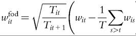
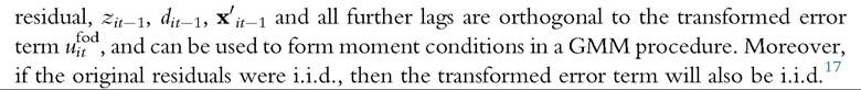
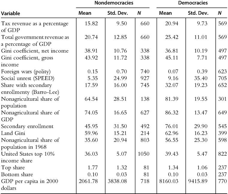
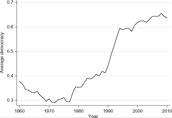
Our estimation framework controls for two key sources of potential bias. First, it controls for country fixed effects, which take into account that democracies are different from nondemocracies in many permanent characteristics that we do not observe and that may also affect inequality and taxation.[379] [380] Second, it allows for mean-reverting dynamics and persistent effects in the dependent variable that may be endogenous to democracy. This focus on changes in democracy ignores variation across countries that never change political institutions, for example, the United States, India, and China, but these observations help us in forming the counterfactual outcome conditional on the right-hand side covariates. Put differently, countries that never change political institutions may still be informative about how taxation and inequality change as a function of past taxation and inequality. The simplest way of estimating Equation (21.6) is by OLS and imposing ρ = 0, and this is the most common regression in the prior literature which has used panel data. But, as already pointed out above, if ρ > 0, this specification may lead to biased estimates and will not correctly identify the long-run effect of democracy on the outcome of interest. Our preferred estimation strategy is to deal with this econometric problem using a standard generalized method of moments (GMM) estimator along the lines of Holtz-Eakin et al. (1988) and Arellano and Bond (1991). This involves differencing Equation (21.6) with respect to time where Tit is the number of times wis appears in the data for s > t. Forward orthogonal differences also remove the fixed effects. In the absence of serial correlation in the original We will implement this using Arellano and Bond’s GMM estimator with different subsets of moments, and after taking first differences or forward orthogonal differences of the data. As Newey and Windmeijer (2009) show, using the full set of moments in two-step GMM may lead to the “too many instruments” bias, since the number ofpoten- tial moments one could use to estimate the dynamic panel model is quadratic in the time dimension. Thus, we experiment by restricting the number of lags used to form moments in the estimation. 17 Estimates of the model obtained by taking forward orthogonal differences are different from the first difference estimates only in unbalanced panels or when not all Arellano and Bond moments are used, in which case different lags give different moments and these may match dynamics differently.Yet another alternative is Blundell and Bond’s (2000) system GMM, which works with the level equation (rather than the difference equation as in Equation 21.7 above) and uses first differences of the dependent variable as instruments for the lagged level. For consistency, this estimator thus requires that the initial value of the dependent variable, in this case democracy, is uncorrelated with the fixed effects. This is unlikely to be a good assumption in our context given the historically determined nature of both democracy and inequality/redistribution. one-step GMM estimators with a naive weighting matrix that assumes the original residuals are i.i.d.18 Despite the potential loss in efficiency, these estimators have the advantage of being consistent when T (the time dimension of the panel) and N (the number of countries) are large, even if the number of moments also becomes large (see Alvarez and Arellano, 2003). As the above description indicates, the source of bias in the estimation of Equation (21.6) with OLS is that the persistence parameter ρ is not estimated consistently when the time dimension does not go to infinity, and this bias translates into a bias in all other coefficient estimates. If we knew the exact value of ρ and could impose it, the rest of the parameters could be estimated consistently by OLS. Motivated by this observation, we also report OLS estimates of Equation (21.6) imposing a range of values of ρ, which shows that our main results are robust to any value of ρ between 0 and 1, increasing our confidence in the GMM estimates. In all cases, we first focus on results using a 5-year panel, where we take an observation every 5 years from 1960 to 2010. This is preferable to taking averages, which would introduce a complex pattern of serial correlation, making consistent estimation more difficult. The 5-year panel is a useful starting point since we expect many of the results of democracy on the tax to GDP ratio (henceforth, short for tax revenue as a percentage of GDP) and inequality not to appear instantaneously or not even in one or two years. In the case of inequality measures, this is also the highest frequency we can use.[381] [382] For the tax to GDP ratio, the annual data are available, and we also estimate annual panels, which are similar to Equation (21.6) except that in that case we include up to 12 annual lags of both the lagged dependent variable and the democracy measure on the right-hand side. Finally, it is worth reiterating that in all of our estimates, if democracy is correlated with other changes affecting taxes or inequality, our estimates will be biased. The point of the GMM estimator is to remove the mechanical bias resulting from the presence of fixed effects and lagged dependent variables, not to estimate “causal effects.” This would necessitate a credible source of variation in changes in democracy, which we do not use in this paper. 21.4.2 Data and Descriptive Statistics We construct a yearly and a 5-year panel of 184 countries from independence or 1960, whichever is later, through to 2010, though not all variables are available for all countries in all periods. We extend the recent work by Papaioannou and Siourounis (2008) by constructing a new measure of democracy which combines information from Freedom House and Polity IV—two of the more widely used sources of data about political rights and democracy. We create a dichotomous measure of democracy in country c at time t, dct, as follows. First, we code a country as democratic during a given year if Freedom House codes it as “Free” or “Partially Free,” and it receives a positive Polity IV score. If we only have information from one of Polity or Freedom House, we use additional information from Cheibub et al. (2010, henceforth CGV) and Boix et al. (2012, henceforth BMR). In these cases, we code an observation as democratic if either Polity is greater than 0, or Freedom House codes it as “Partially Free” or “Free” and at least one of CGV or BMR code it as democratic. We are interested in substantive changes in political power, and so we give priority to the expert codings of Polity and Freedom House, rather than the procedural codings of CGV and BMR. We omit periods where a country was not independent. Finally, many of the democratic transitions captured by this algorithm are studied in detail by Papaioannou and Siourounis (2008), who code the exact date of the democratization. When we detect a democratization that is also in their sample (in the same country and generally within 4 years of the year obtained by the previous procedure), we modify our democracy dummy to match the date to which they trace back the event using historical sources. The Papaioannou and Siourounis measure of democracy captures permanent changes in political institutions, and they find that this correlates with subsequent economic growth. One limitation of their measure is that they define permanent changes by looking at democratizations that are not reversed in the future, which raises the possibility of endogeneity of the definition of democracy to subsequent growth or other outcomes that stabilize democracy. In addition, it means that they have no variation coming from transitions from democracy to autocracy. Our measure retains the focus on large changes in political regimes while not using any potentially endogenous outcome to classify democratizations. Our resulting democracy measure is a dichotomous variable capturing large changes in political institutions. Our sample contains countries that are always democratic (dct = 1 for all years) like the United States and most OECD countries; countries that are always autocratic (dct = 0 for all years) like Afghanistan, Angola, and China; countries that transition once and permanently into democracy like Dominican Republic in 1978, Spain in 1978, and many ex-Soviet countries after 1991. But different from Papaioannou and Siourounis, we also have countries that transition in and out of democracy such as Argentina, which is coded as democratic from 1973 to 1975, falls back to nondemocracy and then democratizes permanently in 1983. For more details on our construction of the democracy measure, see Acemoglu et al. (2013a). In AppendixB, we show robustness of our main results to other measures of democracy constructed by Cheibub et al. (2010) and Boix et al. (2012). We combine this measure of democratization with national income statistics from the World Bank economic indicators. We use government taxes to GDP and revenues to GDP ratios measures obtained from Cullen Hendrix covering more than 127 countries yearly from 1960 to 2005 (Hendrix, 2010). These data come from a project now updated by Arbetman-Rabinowitz et al. (2011), and puts together in a consistent way information from the World Bank (for 1960—1972), the IMF Government Financial Statistics historical series, the IMF new GFS, and complementary national sources.[383] Other dependent variables we explored include secondary-schooling enrollment, agricultural shares of employment, and GDP from the World Bank; and our inequality data that will be described below.[384] Our additional covariates include a measure of average intensity of foreign wars over the last 5 years, constructed from Polity IV and ranging from 0 (no episodes) to 10 (most intense episodes); a measure of social unrest from the SPEED project at the University of Illinois averaging the number of events over the last 5 years;[385] and the fraction of the population with at least secondary schooling from the Barro-Lee dataset. In order to explore interactions we use data on the nonagricultural share of employment in 1968 from Vanhanen (2013).[386] We also use the top 10% share of income in the United States from the World Top Incomes Database (Alvaredo et al., 2010). [387] Finally, we construct the average ratio between the share of income held by the top 10% relative to the bottom 50%, and the ratio between the share of income held by the bottom 10 relative to the bottom 50% before 2000 using the World Inequality Indicators Database. From now on we will refer to these measures as the top and bottom shares of income.[388] There is some debate on the construction and standardization of inequality measures, particularly Gini coefficients, across countries. We use the data in the Standardized World Inequality Indicators Database (SWIID), constructed by Frederick Solt (Solt, 2009). This database uses the Luxembourg Income Study together with the World Inequality Indicators Database in order to construct a comprehensive cross-national panel of Gini coefficients that are standardized across sources and measures. One advantage of this dataset is that it provides both the net Gini, after taxes and transfers, and the gross Gini coefficients. Measuring country-level inequality is very data-demanding, and so no inequality database is completely satisfactory, but we believe the SWIID provides the most comprehensive and consistent measure for the panel regressions we are estimating. We have experimented with a number of other measures of Gini coefficients, but none have the standardized sample coverage of the SWIID. In particular, we also created a panel with data every 5 years using observations for the Gini coefficient from the World Income Inequality Database (WIID) and CEDLAS (for Latin American countries), and obtained very similar results. Descriptive statistics for all variables used in the main sample are presented in Table 21.1, separately by our measure of nondemocracy and democracy (observations in a country that was nondemocratic at the time or democratic). In each case, we report means, standard deviations, and also the total number of observations (note that our Table 21.1 Summary statistics Note: Summary statistics broken by observations during nondemocracy (left panel) and democracy (right panel). See the text for a full description of the data. sample is not balanced). The summary statistics show that democracies tend to be significantly more economically developed than nondemocracies, with much higher GDP per capita, more education, and smaller agricultural shares of employment (both on average in the sample and in 1968) and GDP. These patterns are relatively well known and are sometimes interpreted as support for modernization theory (but see Acemoglu et al., 2008, 2009 on why this cross-sectional comparison is misleading). The differences in tax to GDP ratios and revenue to GDP ratios are much smaller; both variables are roughly 4 percentage points higher in democracies than nondemocracies, although not significantly so.[389] Consistent with this tax difference reflecting increased redistribution, after-tax inequality, measured by the net Gini, is almost three points lower in democracies, whereas pretax inequality is one point higher (the Gini is measured on a 0- to 100-scale). Figure 21.1 shows the evolution of average democracy in our sample between 1960 and 2010.[390] Figure 21.1 Worldwide average democracy since 1960. 21.5.