ESTIMATING THE GLOBAL DISTRIBUTION OF INCOME
In this section we present new estimates of the global distribution of income that combine household survey data with top income data. These estimates are constructed from Milanovic’s (2012) global distribution data set of household surveys for five “benchmark” years in the period 1988—2005, which we have supplemented with top income estimates from income tax data.
Milanovic’s data are provided in quantiles, in most cases 20 income groups each comprising 5% of the population. For those countries for which Milanovic (2012, pp. 10—11) has unit record data, he compared inequality based on individual records with that based on the constructed vigintile (5%) shares and found that the underestimation of the Gini using vigintile shares varied from 0.001 to 0.006 with a mean of 0.003. We agree with Milanovic that this is small enough to be inconsequential.The five benchmark years 1988, 1993, 1998, 2002, and 2005 each have surveys for between 103 and 124 countries and cover between 87% and 92% of the world population and between 95% and 98% of global GDP in PPP$. The Milanovic data set provides incomes in national currencies, which we convert to our numeraire of international dollars using World Bank PPPs.[674] We thus have incomes from household surveys in PPP$ for 87% of the world population in 1988, and 90—92% in the later years. There are 67 countries for which we have both survey and PPP data in all five benchmark years, which we refer to as the “common sample over time”.
As seen in Table 11.2, we have a total of 537 country-years in our data set. Ofthese, 104 country-years, ranging from 18 to 23 countries in each year, also have income tax data on the share of the top percentile of the population, which we downloaded from the World Top Incomes Database.[675] These countries include the three largest developing countries—China, India, and Indonesia; one Latin American country—Argentina; one African country—South Africa; and all the G7 countries.
The rationale for using income tax data for top percentile shares is that household surveys typically fail to capture the incomes of the richest members of society. For example, Szekely and Hilgert (1999) found that in most surveys in Latin America the richest
Table 11.2 Coverage of countries and populations with both household surveys and PPP data, 1988-2005
| Year | Number of countries | Population in billions (% of world population) |
| 1988 | 92 | 4.45 (87) |
| 1993 | 104 | 5.06 (91) |
| 1998 | 109 | 5.32 (90) |
| 2002 | 113 | 5.78 (92) |
| 2005 | 119 | 5.95 (92) |
| Total | 537 |
Source: Authors' calculations.
individuals had an income no higher than what would be expected of a midlevel manager in an international firm. This suggests that very rich households are simply excluded from surveys, which is the assumption we make in incorporating top income data into our survey distributions. In other words, we assume that the survey data in the Milanovic data set represent only the bottom 99% of the population in each country. Accordingly we multiply the population in each income group in the surveys by 0.99 and append the top percentile with its income share from the tax data (assuming that its share of “control” income is equal to its share of survey income). The exclusion of the top percentile implies that mean income in the surveys is underestimated, and our procedure results in a corresponding increase in mean income for each country.
For those country-years that do not have top income data, we impute top percentile shares on the basis of regression. The income share of the top decile in Milanovic's household survey data is strongly correlated with the income share of the top percentile in the independently estimated top income data. Excluding one visible outlier in the 104 country-years with both Milanovic data and top income data,[676] the simple OLS regression coefficient of the income share of the top percentile against the income share of the top decile (on the remaining 103 datapoints) has a t-statistic of7.46 and an R2 of0.36. We then added the original mean income from the surveys as a further regressor. Mean income is found to be highly significant with a /-statistic of 6.69, the top decile share becomes still more significant with a /-statistic of 10.33, and the regression R2 rises to 0.55.[677] We use this latter regression to generate predicted values for the income share of the top percentile for country-years without tax data.
Lakner and Milanovic (2013) take a different approach to imputing top income shares in estimating global inequality between 1988 and 20 08.[678] Following Banerjee and Piketty’s (2010) finding in India that a significant part of the discrepancy between estimates of consumption expenditure in the national accounts and in household surveys can be accounted for by missing or underreported top incomes, Lakner and Milanovic attributed the difference between HFCE and survey incomes (when the former is larger than the latter) entirely to the top decile of the national distribution in each country-year, and add this residual to the income of the top decile reported in the survey. They then calculated a Pareto coefficient for each country-year distribution on the basis of the unadjusted survey income in the ninth decile and the adjusted income in the top decile (following the procedure described in Atkinson, 2007).
Assuming this Pareto distribution applies within the top decile of each country-year distribution, they estimated income shares for the income groups P90—P95 (i.e., percentile 90 to percentile 95), P95—P99, and P99—P100, yielding 12 income groups per country-year.An implicit assumption behind Lakner and Milanovic’s procedure for imputing top incomes is that HFCE per capita is the correct measure of mean consumption expenditure (or income), when it is larger than the corresponding survey mean. We have argued against using national accounts means in Section 11.4 and in Anand and Segal (2008). It should also be noted that Milanovic’s (2002, 2005, 2012) own previous estimates of “true” global inequality are based on his assumption that survey means are preferable to national accounts means.
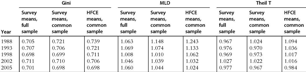
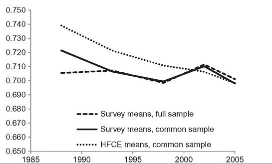
11.5.1 Global Inequality Estimates With and Without Top Income Data
Our results for global inequality are presented in Table 11.3 and Figure 11.1. The first notable finding is the very high level of global inequality. Considering the global distribution with top incomes over the period 1988—2005, the Gini varies between 0.722 and 0.735, MLD (or Theil L) between 1.093 and 1.156, and Theil T between 1.114 and 1.206. The top percentile in the world has a share between 17.3% and 20.7% of global income, and the top decile between 58.5% and 62.0%. The richest percentile in the world have mean incomes almost 21 times the world mean income in 2005, or a mean per capita household income of about PPP$90,000 in 2005. The threshold for being in the top percentile in 2005 was PPP$42,000.[679]
As anticipated, the inclusion of top income data raises the estimated levels of inequality relative to those based on household surveys without top income data. The average
Table 11.3 Global inequality with and without top incomes, 1988-2005
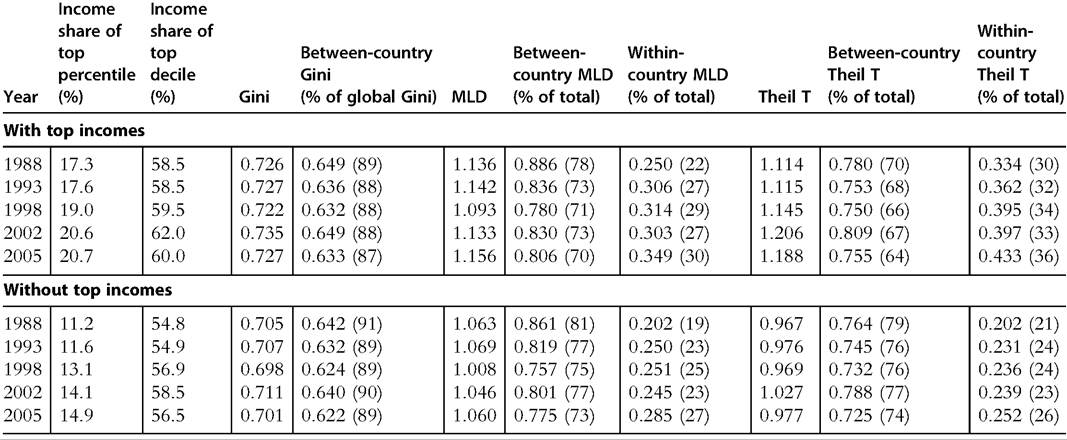
Source: Authors' calculations.
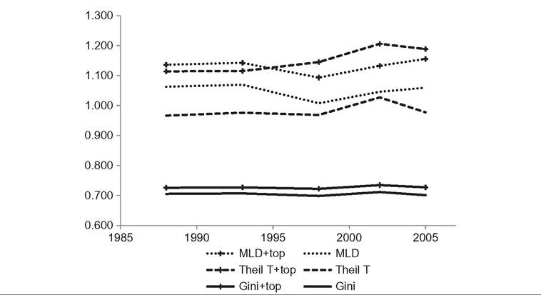
Figure 11.1 Global inequality with and without top incomes, 1988-2005.
Note: Estimates with top income data included are denoted “+topquot;. Source: Table 11.3.share of the top percentile over the period 1988—2005 increases from 13.0% on the basis of the surveys alone to 19.0% when top income data are included. Correspondingly, the average top decile share over the period is 56.3% with survey data alone, and 59.7% when top income data are added. Depending on the year, the Gini increases by 3—4%, MLD (or Theil L) by a larger margin of 7—9%, and Theil T by the largest margin of 14—22%. For all measures the increase is greatest in 2005, when the inclusion of top income data raises the global Gini by 4%, MLD by 9%, and Theil T by 22%. These differences in impact reflect the different sensitivities of the measures to income changes at the top end of the distribution.
Turning to changes in inequality with top income data during 1988-2005, the income share of the top percentile rises monotonically from 17.3% to 20.7%. The share of the top decile rises from 58.5% in 1988 to 60.0% in 2005, peaking at 62% in 2002. The Gini coefficient shows very little movement in this period: the highest Gini value is 0.735 (in 2002), which is only 0.013 higher than the lowest Gini value of 0.722 (in 1998), a difference of under 2%. MLD (or Theil L) and Theil T show somewhat larger movements, with the difference between the highest and lowest years for the measures being 6% and 8%, respectively. MLD peaks in 2005 and Theil T in 2002, and for both of these measures inequality rises over the period 1988-2005—for MLD by 1.8% and for Theil T by 6.6%.
The top income data modify both the estimated level of global inequality and its rate of change over time. Although inequality rises over 1988-2005 according to MLD and Theil T with top income data included, inequality is virtually unchanged over the period according to all three measures when top income data are not included. In the latter case the Gini is 0.705 in 1988 and 0.710 in 2005, MLD is virtually unchanged at 1.06, and Theil T rises marginally from 0.967 to 0.977; however, the income share of the top percentile rises from 11.2% to 14.9%.
The changes in inequality over time are not large compared to changes witnessed in some individual countries. This is particularly so in the case of the Gini coefficient, where the peak-to-trough difference is only 1.3 Gini points with the top income data, compared to a rise, for example, of about 5 Gini points in the United States over the period 1988—2005.2 Moreover, given the different sources of estimation error that we described in Section 11.4, the small changes we find in the global inequality indices may not be statistically significant—particularly in the cases of the Gini and MLD, which are less than 2 percentage points different in 2005 from 1998. However, the rise in the share of the global top percentile, from 17.3% to 20.7% during 1988—2005, seems less trivial; it implies that the incomes of the top percentile increased by 20% relative to mean income—though we note that this is also smaller than the rise in the share of the top percentile in the United States over the same period, from 15.5% to 21.9%.[680] [681] In the Appendix we provide analogous results for the “common sample over time” of 67 countries. Whereas the full sample shown earlier comprises between 87% and 92% of the world population depending on benchmark year, the common sample over time comprises between 79% and 82%. As can be seen in Appendix Table 11.A2, the global inequality estimates are very similar to those in Table 11.3 shown earlier. The Gini coefficient for the common sample is never more than 1 percentage point different from that for the full sample, whereas MLD and Theil T are never more than 3 percentage points different. Note that the common sample over time is not necessarily more representative of the global income distribution than our full sample in each benchmark year, and estimates of the level or rate of change of global inequality based on the common sample are not necessarily more accurate. Our calculations with top income data assume that household surveys do not capture the top percentile of the national income distribution. An alternative way to include the top income data is to assume that surveys are indeed representative of all households, but that they underreport the incomes of the top percentile in the national distribution. This is the assumption made by Alvaredo and Londoilo Velez (2013) and requires a different calculation. Rather than multiply the population of each income group in the survey data by 0.99 and then append the top percentile with its income share from the tax data, on the alternative assumption one simply replaces the income of the top percentile in the survey data with that from the tax data. We have performed this calculation as well, and it leads to marginally lower estimates of global inequality: in the five benchmark years the global Gini is upto 0.4% smaller, and MLD and Theil T are upto 1.2% smaller. However, for the latter two decomposable indices, the within-country component is noticeably smaller, by 3.6-5.2% for MLD and by 2.4-4.1% for Theil T—but the between-country component is about 0.5% larger for both indices. 11.5.2 Comparison OfAlternative Estimates of Global Inequality We saw earlier that only three previous studies have used 2005 PPPs to estimate global inequality: Bourguignon (2011), Milanovic (2012), and Lakner and Milanovic (2013). Milanovic’s (2012) estimates of global inequality are directly comparable to our estimates without top incomes in Table 11.3, as they are based on the same survey data and methodology. The only substantial difference we know of is in the PPPs used for countries for which the World Bank does not have data (see footnote 23 for the sources that we use in these cases). Milanovic found the Gini coefficient to vary between 0.684 and 0.707 in the period 1988-2005, whereas in our estimates given earlier it varies between 0.698 and 0.711. However, whereas we find Theil T at virtually the same level in 1988 as in 2005, he found it to rise from 0.875 to 0.982 over the same period. Lakner and Milanovic (2013), like us, estimated global inequality both with and without imputed top incomes. Their estimates without top incomes also follow the same methodology as Milanovic (2012) and are based directly on survey data. Lakner and Milanovic’s estimates of the global Gini without top incomes are close to ours, varying between 0.705 and 0.722 in the period 1988-2008. Their Theil T is slightly higher than ours, varying between 1.003 and 1.049 in the period. Significantly, their MLD shows a marked decline, from 1.142 in 1988 to 1.027 in 2008. Lakner and Milanovic—like us—found that imputing top incomes leads to higher estimates of global inequality. Their HFCE-based method of imputing top incomes, discussed earlier, raises the global Gini by 3.8-6.3 Gini points, with the difference rising over time in the period 1988-2008.[682] Nonetheless, their Gini ends the period at almost exactly the same level as it began, declining marginally from 0.763 in 1988 to 0.759 in 2008. This is a much larger effect than we find from adding top income data to the survey data. As we saw in Table 11.3, our method leads to the Gini being approximately 2 Gini points higher in each year. Lakner and Milanovic themselves pointed out that their imputation assumption is rather extreme in some cases. For example, in 2008 in India—the country that appears to have motivated their procedure—they find the survey mean to be only 53% of HFCE per capita, so they attribute the remaining 47% of total HFCE entirely to the top decile, adding it to the income of the top decile reported in the survey. This adjustment seems implausibly large to us. Conversely, for China in both 1988 and 2008, HFCE is smaller than survey income, so no adjustment is made by the authors for underreporting or undersampling of top incomes. 31 The final study that uses 2005 PPPs to estimate global inequality is Bourguignon (2011), which—unlike the other studies mentioned in this section—scales within- country distributions to GDP per capita. Bourguignon found the Gini coefficient to decline from approximately 0.70 to 0.66 between 1989 and 2006 (these numbers were read off his Figure 1). This is a substantial decline compared with the findings reviewed earlier of virtually no change in the Gini without top incomes. The main difference between Bourguignon’s estimates and the other estimates without top incomes discussed here is that Bourguignon scales to national accounts data. In Section 11.4 we argued that if one uses national accounts data then HFCE is preferable to GDP as an approximation to household income, so we compare estimates based on survey means with estimates based on HFCE means in the next section. 11.5.3 Global Inequality Estimates Using NA Means, Without Top Income Data In this section we report global inequality estimated by scaling household survey incomes so that the scaled mean is equated to per capita HFCE from NA in each country (in contrast to using incomes directly from the surveys). HFCE figures in PPP$ are not available for all the country-years for which we have household survey data. In each year, we distinguish between the “full sample” defined as the set of all countries with survey data, and the “common sample” across data sets defined as the subset of the full sample countries that also have HFCE data in PPP$ (note that this is different from the “common sample over time,” defined earlier). In 1988 the common and full samples are quite different: in that year the countries that have both survey data and HFCE data in PPP$ comprise only 77% of the world population, compared with 87% of the world population for countries in the full sample (see Table 11.2).[683] In the other years covered in Table 11.2, the common sample has 3-4% less of the world population than the full sample.[684] For each of our indices, Table 11.4 presents three different global inequality estimates without top income data: first, the full sample estimates as in Table 11.3; second, estimates based on survey data restricted to the common sample; and third, the common sample estimates based on per capita HFCE (as described earlier). We will refer to the first as the Table 11.4 Global inequality estimates using survey means and HFCE means, without top incomes, 1988-2005 Note: Full sample consists of all countries for which household survey data are available, as in Tables 11.2 and 11.3. Common sample in a given year consists ofthe subset of countries with both survey data and HFCE data in PPP$ in that year. Source: Authors' calculations. full sample survey-means estimates, the second as the common sample survey-means estimates, and the third as the common sample HFCE-means estimates. This highlights the fact that in the first two, mean incomes in each country are obtained directly from the surveys, whereas in the third the mean is externally imposed from HFCE data. These estimates exclude the top income data so that we can focus on the differences in global inequality using survey and NA mean incomes. Figure 11.2 plots the Gini coefficients for the three different sets of data. The most notable difference between the full sample survey-means estimates and the common sample HFCE-means estimates is that whereas the former appear relatively flat, the latter have a clear downward trend. The two estimates are approximately the same in 2002 and 2005, but because of their different starting points in 1988 the full sample survey-means Gini declines by only 0.004 between 1988 and 2005, from 0.705 to 0.701, whereas the common sample HFCE-means Gini declines by 0.041, from 0.739 to 0.698. However, the common sample survey-means estimates indicate that about half this difference is explained by the difference between the full and common sample: the common sample survey-means Gini declines by 0.023, from 0.721 to 0.698. The second factor that appears to explain the difference in trend for the HFCE-means Gini and the survey-means Gini is the divergent trend for India specifically in comparing survey and HFCE means, a phenomenon that has been examined in detail by Deaton and Kozel (2005). In our data the average annual growth rate of per capita household consumption expenditure in India from 1988 to 2005 was 2.8% according to surveys, and more than twice that at 5.8% according to HFCE from the National Accounts. When we both restrict the estimates to the common sample and exclude India from it, the survey-means Gini declines by 0.029, whereas the HFCE-means Gini decreases by a Figure 11.2 Global Gini without top incomes, using survey means and HFCE means, 1988-2005. Note: Common sample consists of surveys restricted to country-years with HFCE data. Source: Table 11.4. similar magnitude of 0.034.[685] Thus ensuring a common sample and excluding India virtually eliminates the difference in trend between HFCE-means and survey-means estimates of the Gini.[686] Thus the divergence between HFCE-means and survey-means estimates seems to be due to the loss of as much as 10% of the world population in the “common sample” that has both survey and HFCE data, and the divergent trends in India. Given this, in our view the decline in global inequality implied by the HFCE calculations is likely to be illusory. We have not examined estimates based on GDP means, as opposed to HFCE means, for the reasons mentioned earlier. Still, these findings do not seem to corroborate Bourguignon’s (2011) result for the period 1989-2006, based on GDP data and discussed earlier, that “inequality decreases, and it decreases at a very fast pace.” 11.6.