Generalized Linear Models
Our exposition of GLMs draws on Nelder and Wedderburn (1972), McCullagh and Nelder (1989), and Firth (1991). We treat GLMs in an applied manner covering the basic structure of the models, estimation, and model fitting.
We do not provide a detailed exposition of the method itself. Readers interested in a complete statistical treatment of GLMs can refer to McCullagh and Nelder (1989) or to Dobson (2001). The former presents an excellent and comprehensive statistical overview of GLMs, but assumes an advanced statistics background on the part of the reader. The latter presents a briefer and more synthetic exposition of GLMs at a moderate level of statistical complexity.Generalized linear models are an extension of classic linear models. The linear regression model has found widespread application in the social sciences mainly due to its simple linear formulation, easy interpretation, and estimation. In monetary poverty analysis, linear regression analysis has been used to study the determinants of household consumption expenditures or to model the growth elasticity of per capita income or income poverty aggregates like the headcount ratio or the poverty gap index.[250] Linear regressions are also used to model changes in (i) the income share of the poorest quintile (Dollar and Kraay 2004); (ii) adjusted GDP incomes (Foster and Szdkely 2008); (iii) the poverty rate (Ravallion 2001); and (iv) the growth rates of real per capita GDP (Barro 2003).
10.2.1 Classiclinearregression
We begin with a brief review of the classic linear regression model and its notation and build on this to present the more generic case of GLMs. The classic linear regression model (LRM) assumes that the endogenous or dependent variable (y) (hitherto referred to as ‘endogenous') is a linear function of a set of K exogenous10 variables (x).
The LRM assumes that the endogenous variable y is continuous and distributed with constant variance. In addition, the LRM may also assume that the endogenous variable is normally distributed. However, this assumption is not needed for estimating the model but only to obtain the exact distribution of the parameters in the model. In the case of large samples one may not need to assume normality in an LRM as inference on parameters is based on asymptotic theory (cf. Amemiya 1985). These assumptions may be inappropriate if the endogenous variable is discrete (binary or categorical)—or continuous but non-normal.11 GLMs overcome these limitations. They extend classic linear regression to a family of models with non-normal endogenous variables. In what follows, random variables are denoted in upper-case and observations in lower-case; vectors are represented with lower-case bold and matrices with upper-case bold.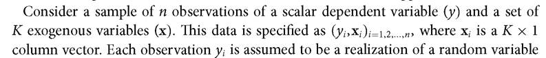
Yi independently distributed with mean μγi. The classic regression model with additive errors for the ith observation can be written as
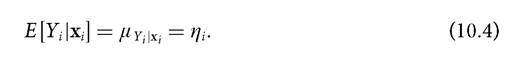
where E [Yi ∣xi] denotes the conditional expectation12 of the random variable Yi, given xi, and εi is a disturbance or random error. From equation (10.1) we see that the dependent variable is decomposed into two components: a systematic or deterministic component given the exogenous variables and an error component. The deterministic component is the conditional expectation E [Yi ∣xi], while the error component, attributed to random variation, is εi.
Equation (10.1) is a general representation of regression analysis. It attempts to explain the variation in the dependent variable through the conditional expectation without imposing any functional form on it.
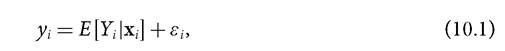
If we specify a linear functional form of the conditional expectation E [Yi ∣xi], we obtain the classic linear regression model. Then, the systematic part of the model may be written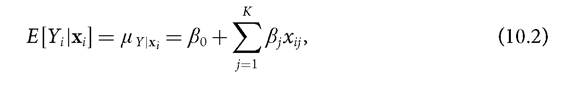
10 In the statistical literature x is referred to as a ‘regressor’ or ‘covariate’ that is exogenous when the assumptions on the disturbance term are conditional on the covariates. In our exposition, all assumptions on the disturbance term or the dependent variable are conditional on the regressors so we use the term ‘exogenous’ instead of the generic term ‘regressor’. By ‘exogenous’ we mean non-stochastic or conditionally stochastic right-hand-side variables.
11 An example of a non-normal continuous variable is income (consumption expenditures). The distribution of income is skewed (to the right), takes on only positive values, and is often heteroscedastic.
12 Or conditional mean. We use both terms interchangeably.
where xij is the value of the jth exogenous variable for observation i. To show the relation between a linear regression model and a generalized linear model it will become convenient to denote the right-hand side of equation (10.2) by ηi, referred to as the predictor in the generalized linear model. Thus we can write
and then the systematic part can be expressed as
Equations (10.1) to (10.4) lead to the familiar linear regression model:
j=1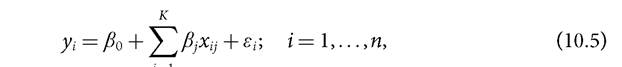
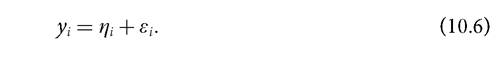
where β0, β1,..., βκ are parameters whose values are unknown and need to be estimated from the data.13 Note that in the linear regression model of equation (10.6), the conditional expectation is equal to the linear predictor:
The LRM additionally assumes that the errors (εi) are independent, with zero mean, constant variance (σ2), and follow a Gaussian or normal distribution.14 Often the assumptions on εi are made conditional on the exogenous variables, as these are possibly stochastic or random.
Then, the errors have zero mean and homoscedastic or identical variance, conditional on the exogenous variables, that is, εi ∣xi ~ N (0, σe2). Due to the relationship between y and ε, the dependent variable is also normally distributed with constant variance. In other words, in an LRM, the distribution of the dependent variable is derived from the distribution of the disturbance. However, as explained in section 10.2.2, in a GLM the distribution of the dependent variable is specified directly.13 An equivalent expression of the LRM is a matrix representation of the form y = Xβ + ε, where y =
T
{y1,...,yn} is an n ? 1 vector of observations; ε is an n ? 1 vector of disturbances; X is a n ? K matrix of explanatory variables, where each row refers to a different observation, each column to a different explanatory T
variable; and β = {β1,..., βκ} is a K ? 1 vector of parameters. However, for the expositional purposes of this chapter we do not use the matrix representation but rather the one specified in equation (10.5).
14 To denote a random variable as normally distributed we follow the statistical convention and denote it as N (∙).
10.2.2 Thegeneralization
The GLM family of models involves predicting a function of the conditional mean of a dependent variable as a linear combination of a set of explanatory variables. Classic linear regression is a specific case of a GLM in which the conditional expectation of the dependent variable is modelled by the identity function. GLMs extend the domain of applicability of classic linear regression to contexts where the dependent variable is not continuous or normally distributed. GLMs also permit us to model continuous dependent variables that have positively skewed distributions.
Generalized linear models relax the assumption of additive error in equation (10.1).
The random component is now attributed to the dependent variable itself. Thus, for GLMs we need to specify the conditional distribution of the dependent variable, given the values of the explanatory variables, denoted as fγ (y). These distributions often belong to the linear exponential family, such as the Gaussian, binomial, poisson, and gamma, among others, but have also been extended to non-exponential families (McCullagh and Nelder 1989).A generalized linear model is one that takes the form:
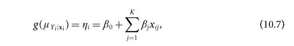
where the systematic part or linear predictor (ηi) is now a function (g) of the conditional expectation of the dependent variable μ γ∙i∣xi; g(∙) is a one-to-one differentiable function referred to as the link function; and η is referred to as the linear predictor. The link function transforms the conditional expectation of the dependent variable to the linear predictor, which is a linear function of the explanatory variables that could be of any nature. This allows the linear predictor to include continuous or categorical variables, a combination of both, or interactions—as well as transformations of continuous variables. Note that when the link function g(∙) is the identity function, we have an LRM.
In most applications, as in the regression analysis with AF measures, the primary interest is the conditional mean μ Yi ∣xi. This could be easily retrieved from equation (10.7) by inverting the link function; hence we can write
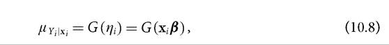
where G(∙) is the inverse linkg-1 (∙), also called the mean function. Equations (10.7) and (10.8) provide two alternative specifications for a GLM, either as a linear model for the transformed conditional expectation of the dependent variable—given by (10.7)—or as a non-linear model for the conditional mean—given by (10.8).
A GLM is thus composed of three components: (i) a random component resulting from the specification of the conditional distribution of the dependent variable, given the values of the explanatory variables (ii) a linear predictor ηi; and (iii) a link function g(∙) (cf. Fox 2008: ch. 15).
Table 10.1 Generalized linear regression models with AF measures
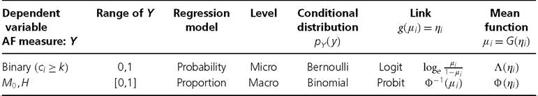
Note: Φ(∙) and Λ(∙) are the cumulative distribution functions of the standard-normal and logistic distributions, respectively. For the binary model, the conditional mean μl is the conditional probability πl.
The distribution of the dependent variable fγ (y) and the choice of the link function are intimately related and depend on the type of variable under study. The form of a proper link function is determined to some extent[251] by the range of variation of the dependent variable and consequently by the range of variation of its conditional mean.
In the case of AF poverty measures, we may consider two types of dependent variables with a different range of variation and distribution. The first type is a binary indicator identifying multidimensionally poor households. This variable takes the value of one if the household is identified as multidimensionally poor and zero otherwise. The Bernoulli distribution is suitable to describe this kind of variable. A typical model in this case is the probit or logit model. As we will see, in a GLM this is equivalent to choosing a logit link. The second type of dependent variable that we could study in the AF approach is a proportion. The Adjusted Headcount Ratio M0 and the incidence H are fractions or proportions that take values in the unit interval. The binomial distribution may be suitable as a model for these proportions.
In each of these cases, the link function should map the range of variation of the dependent variable—{0,1} for the binary indicator and [0,1] for the proportion—to the whole real line (-∞,+∞). The scale is chosen in such a way that the fitted values respect the range of variation of the dependent variable. Columns one to five in Table 10.1 present the two types of dependent variables with AF measures that we study in this section, along with their range of variation, type of model, level of analysis, and random variation described by the conditional distribution. The link and mean functions are explained in the examples in sections 10.3 and 10.4. Before presenting the examples, we briefly explain the estimation and goodness of fit of GLMs.
10.2.3 ESTIMATION AND GOODNESS OF FIT
Once we have selected the particular models of our study, we need to estimate the parameters and measure their precision. For this purpose we maximize the likelihood or log likelihood[252] of the parameters of our data denoted by l[y; μ (β)].[253] The likelihood function of a parameter is the probability distribution of the parameter given μ (β).
To assess goodness of fit of the possible estimates, we use the scaled deviance. This statistic is formed from the logarithm of a ratio of likelihoods and measures the discrepancy, or goodness of fit, between the observed data and the fitted values generated by the model. To assess the discrepancy we use as a baseline the full or ‘saturated’ model. Given n observations, the full model has n parameters, one per observation. This model fits the data perfectly but is uninformative because it simply reproduces the data without any parsimony. Nonetheless it is useful for assessing discrepancy vis-a-vis a more parsimonious model that uses K parameters. Hence in the saturated model the estimated conditional mean μ = y and the scaled deviance is zero. For intermediate models, say with K parameters, the scaled deviance is positive.
The scaled deviance statistic
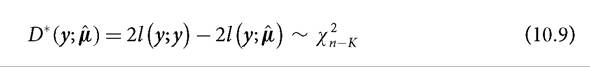
is twice the difference between l (y;y), which is the maximum log likelihood of a saturated model or exact fit, and l (y; μ) the log likelihood of the current or reduced model.
The goodness of fit is assessed by a significance test of the null hypothesis that the current model holds against the alternative given by the saturated or full model. Under the null hypothesis, D* is approximately distributed as a k random variable where the number of degrees of freedom equals the difference in the number of regression parameters in the full and the reduced models. However, an appropriate assessment of the goodness of fit is based on the conditional distribution of D* (y; μ) given β. If D* is not significant, it suggests that the additional parameters in the full model are unnecessary and that a more parsimonious model with lesser parameters may be sufficient.
The scaled deviance statistic is also useful for model selection. Due to its additive property, the discrepancy between nested sets of models can be compared if maximum likelihood estimates are used. Suppose we are interested in comparing two models, A and B, that represent two different choices of explanatory variables, XA and Xb, that are nested. Intuitively this means that all explanatory variables included in model A are also present in model B, a more complex or less parsimonious model. The improvement in fit maybe assessed by a significance test of the null hypothesis that model A holds against the alternative given by model B. If the value of the scaled deviance statistic is found to be significant, there is an improvement in the fit of model B vis-a-vis model A, although a general conclusion on model selection should also consider the added complexity of model B.
10.3