Micro Regression Models with AF Measures
In the case of micro regression analysis, the focal variable is the (household) censored deprivation score ci. This score reflects the joint deprivations characterizing a household identified as multidimensionally poor.
From a policy perspective a natural question that arises consequently is how to understand the ‘causes' that underlie the (multidimensional) poverty status of a household. The simplest model for this purpose is a probability model, which we illustrate in this section; although one could also consider modelling the ci vector directly. We are thus interested in assessing the probability of a household being multidimensionally poor. Within the AF framework this is equivalent to comparing the deprivation score of a household ci with the multidimensional poverty cutoff (k). If ci is above the multidimensional poverty cutoff (k), the household is identified as multidimensionally poor. This is represented by a binary random variable (Yi) that takes the value of one if the household is identified as multidimensionally poor and zero otherwise, as follows:
The outcomes of this binary variable occur with probability πi, which is a conditional probability on the explanatory variables. For a (sampled) household i identified as multidimensionally poor, this is represented as
and thus the conditional mean equals the probability as follows:

For a binary model, the conditional distribution of the dependent variable, or random component in a GLM, is given by a Bernoulli distribution (Table 10.1).
Thus the probability function of Yi is
To ensure that the conditional mean given by the conditional probability stays between zero and one, a GLM commonly considers two alternative link functions (g). These are given by the quantile functions of the standard normal distribution function and the logistic distribution function
 The former is referred to as the probit
link function and the latter as the logit link function. The probit link function does not
18 Note Φ(∙) and Λ(∙) are the cumulative distribution functions of the standard-normal and logistic distribution, respectively.
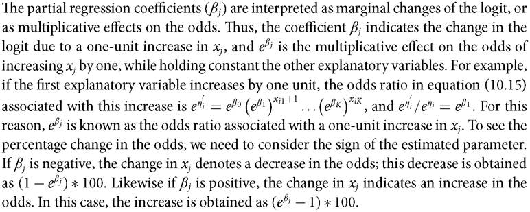
have a direct interpretation, while the logit is directly interpretable, as we will discuss in this section.[254]
The logit of π is the natural logarithm of the odds that the binary variable Y takes a value of one rather than zero. In our context, this gives the relative chances of being multidimensionally poor. If the odds are ‘even'—that is, equal to one—the corresponding probability (π) of falling into either category, poor or non-poor, is 0.5, and the logit is zero. The logit model is a linear, additive model for the logarithm of odds as in equation (10.14), but it is also a multiplicative model for the odds as in equation (10.15):
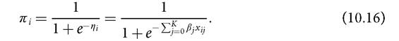
The conditional probability πi is then
ιo.3.ι Amicroregressionexample
To illustrate the type of micro regression models that have been discussed, we use a subsample of the Indonesian Family Life Survey (IFLS) dataset.
This is a dataset analysed by Ballon and Apablaza (2012) to assess multidimensional poverty in Indonesia during the period 1993-2007. The IFLS is a large-scale longitudinal survey of the socioeconomic, demographic, and health conditions of individuals, households, families, and communities in Indonesia. The sample is representative of about 83% of the population and contains over 30,000 individuals living in thirteen of the twenty-sevenTable 10.2 Logistic regression model of multidimensional poverty in West Java
| Variable | Parameter estimate | Robust std. err. | t ratio | Significance level | Odds ratio |
| Years of education of household head | -0.68 | 0.03 | -19.65 | * * | 0.51 |
| Female household head | 0.24 | 0.09 | 2.71 | ** | 1.28 |
| Household size | 0.09 | 0.01 | 7.02 | * * | 1.10 |
| Living in urban areas | -0.85 | 0.07 | -11.40 | ** | 0.43 |
| Being Muslim | -0.02 | 0.32 | -0.07 | n.s. | 0.98 |
** denotes significance at 5% level; n.s. denotes non-significance.
provinces in the country. Ballon and Apablaza (2012) measure multidimensional poverty at the household level in five equally weighted dimensions: education, housing, basic services, health issues, and material resources. For this illustration, we retain a poverty cutoff of 33%.
Thus a household is identified as multidimensionally poor if the sum of the weighted deprivations is greater than 33%. That is, Yi takes the value of one if ci ≥ 33% and zero otherwise. Within the GLM framework this binary dependent variable is estimated by specifying a Bernoulli distribution and a logit link function. This is equivalent to a logit regression.The household poverty profile that we specify regresses the log of the odds of being multidimensionally poor (using k = 33%) on the demographic and socioeconomic characteristics of the household head. For this illustration we use data for West Java in 2007. West Java is a province of Indonesia located in the western part of the island of Java. It is the most populous and most densely populated of Indonesia's provinces, which is why we selected it. The explanatory variables included in this illustration are non-indicator measurement variables and comprise:
• education of the household head, defined as the number of years of education (not necessarily completed);
• the presence of a female household head, represented by a dummy variable taking a value of one if the household head is a female and zero if male;
• household size, defined by the number of household members;
• the area in which the household resides, represented by a dummy variable taking a value of one if the household resides in the urban areas of West Java and zero otherwise;
• Muslim religion, represented by a dummy variable taking a value of one if the household's main religion is Muslim and zero if not.
Table 10.2 reports the logistic regression results of this poverty profile for West Java in 2007. Columns two to five report the estimated regression parameters along with their standard errors, t ratios, and significance levels at 5%.2° Apart from being Muslim, all
20 Note we can also report marginal effects if the interest is to see the effect of an explanatory variable on the change of the probability.
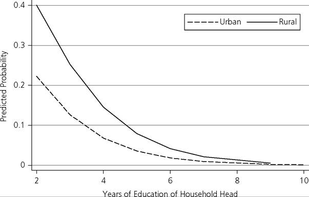
Figure 10.1.
Logistic regression curve—WestJavaother determinants are significant at the 5% level and show the expected signs. For a given household, the log of the odds of being multidimensionally poor decreases with the education of the household head and an urban location, and increases with the presence of a female household head and with household size. The odds ratio for years of education of the household head indicates that an increase of one year of education decreases the odds of being multidimensionally poor by 49%, ceteris paribus, whereas having a female household head increases the odds of being multidimensionally poor by 28%, ceteris paribus.21 Similarly, the odds of a household of being multidimensionally poor decrease by 57% for households living in urban areas, ceteris paribus, and increase by 10% for each additional household member. Figure 10.1 shows the odds model for urban and rural areas as a function of the education of the household head, holding constant the gender status of the household head (female), assuming five household members (average), and being Muslim. The logistic curves show a decrease in the probability of a household being multidimensionally poor as the education of the household head improves. These probabilities are lower for households living in urban areas compared to rural ones.
As religion turns out to be statistically insignificant, we could consider an alternative poverty profile without religion as an explanatory variable (model B). To test whether this restrained model (without religion) is as good as the current model (model A), we compare the deviance statistics of both models.22 Formally we test the following
21 All estimated parameters exhibiting a negative sign denote a decrease in the odds; this is obtained as (1-odds ratio) ? 100. Likewise, estimated parameters with a positive sign denote an increase in the odds; this is obtained as (odds ratio-1)?100. Forthe effect of education we have (1-0.51) ? 100, and for the effect of gender we have (1.28-1) ? 100%.

hypothesis:
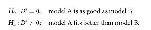
To reject the null hypothesis we compare D* with the corresponding chi-square statistic χ 2df with df degrees of freedom. These degrees of freedom correspond to the difference in the number of parameters in model A and model B. A non-rejection of the null hypothesis indicates that both models are statistically equivalent and thus the most parsimonious model, which has the smaller number of explanatory variables, should be chosen—which is B in this context. A rejection of the null hypothesis indicates a statistical justification for model A. In our case the comparison of the two nested models, A and B, gives a scaled deviance statistic D+ of 0.05. We compare this value with the corresponding chi-square statistic of one degree of freedom and a 5% type I error rate; this gives a value of 3.84. As D+ is smaller than 3.84, we cannot reject the null hypothesis; so we choose the more parsimonious model B and drop religion as an explanatory variable.
10.4