Macro Regression Models for M0 and H
We now turn to the econometric modelling for the Adjusted Headcount Ratio M0 and the incidence of multidimensional poverty H as endogenous or dependent variables. As M0 and H are bounded between zero and one, an econometric model for these endogenous variables must account for the shape of their distribution.
M0 and H are fractional (proportional) variables bounded between zero and one with the possibility of observing values at the boundaries. This restricted range of variation also applies for the conditional mean, which is the focus of our analysis. Thus, specifying a linear model, which assumes that the endogenous variable and its mean take any value in the real line, and estimating it by ordinary least squares is not the right strategy, as this ignores the shape of the distribution of these dependent variables. Clearly if the interest of the research question is not in modelling the conditional mean of the proportion but rather in modelling the absolute change (between two time periods) of M0 or H, which can take any value, standard linear regression models may apply. In what follows we describe the statistical strategy for modelling the conditional mean of M0 or H as a function of a set of explanatory variables.Various approaches have been used in the literature to model a fraction or proportion. We can differentiate between two types of approaches—often referred to as one-step or two-step approaches. These differ in the treatment of the boundary values of the fractional dependent variable. In a one-step approach, one considers a single model for the entire distribution of the values of the proportion, where both the limiting observations and those falling inside the unit interval are modelled together. In a two-step approach, the observations at the boundaries are modelled separately from those falling inside the unit interval.
In other words, in a two-step approach one considers a two-part model where the boundary observations are modelled as a multinomial model and remaining observations as a fractional one-step regression model (Wagner 2001; Ramalho, Ramalho, and Murteira 2011). The decision whether a one- or a two-part model is appropriate is often based on theoretical economic arguments. Wagner (2001) illustrates this point. He models the export/sales ratio of a firm and argues that firms choose the profit-maximizing volume of exports, which can be zero, positive, or one. Thus the boundary values of zero or one may be interpreted as the result of a utility-maximizing mechanism. Following this theoretical economic argument he specifies a one-step fractional model for the exports/sales ratio. In the absence of an a priori criteria for the selection of either a one- or two-part model, Ramalho et al. (2011) propose a testing methodology that can be used for choosing between one-part and two-part models. In the case of M0 or H we consider that non-poverty and full poverty, the boundary values, as well as the positive values, are characterized by the same theoretical mechanism. This is thus represented by a one-part model. For further references on alternative estimation approaches for one-part models, see Wagner (2001) and Ramalho et al. (2011).10.4.1 MODELLING M0 OR H
To model M0 or H we follow the modelling approach proposed by Papke and Wooldridge (1996). For this purpose we denote the Adjusted Headcount Ratio or the incidence by y. For a given spatial aggregate, say a country, the Adjusted Headcount Ratio or the incidence is yi. Papke and Wooldridge (PW hereafter) propose a particular quasi-likelihood method to estimate a proportion. The method follows Gourieroux, Monfort, and Trognon (1984) and McCullagh and Nelder (1989) and is based on the Bernoulli log-likelihood function which is given by
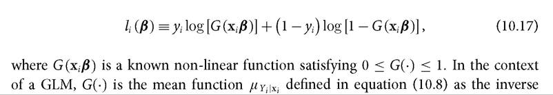
link function.
PW suggest as possible specifications for G(∙) any cumulative distribution function, with the two most typical examples being the logistic function and the standard normal cumulative density function as described in Table 10.1.The quasi-maximum likelihood estimator (QML) obtained from equation (10.17) is consistent and asymptotically normal, provided that the conditional mean μγ. ∣x. is correctly specified. This follows the QML theory where consistency and asymptotic normality characterize all QML estimators belonging to the linear exponential family of distributions, which is the case of the Bernoulli distribution of equation (10.17).
10.4.2 ECONOMETRIC ISSUES FOR AN EMPIRICAL MODEL OF M0 OR H
We would like to conclude with a few recommendations for performing a macro regression with M0 or H as endogenous variables. First, we suggest testing for linearity before specifying a non-linear functional form. For this purpose one can apply the Ramsey RESET[255] test of functional misspecification. The test consists of evaluating the presence of non-linear patterns in the residuals that could be explained by higher-order polynomials of the dependent variable. Second, we recommend testing for possible endogeneity using a two-stage or instrumental variable (IV) estimation. In regressions of the type of the macro determinants of M0 or H, it is very likely that there will be a correlation between one or more of the explanatory variables and the error term. Let us suppose we regress the Adjusted Headcount Ratio on the logarithm of the per capita gross national income in PPP of the same year for a group of countries. This is the GNI converted to international dollars using purchasing power parity rates. This gives a contemporaneous model for the semi-elasticity between growth and poverty. In this very simple model, it is highly likely that the GNI would be correlated with the disturbance of the equation, which consists of unobserved variables affecting the poverty rate.
This violates a necessary condition for the consistency of standard linear estimators. To deal with endogeneity, often one uses an instrumental variable that is assumed to be correlated with the endogenous explanatory variable but uncorrelated with the error term.Third, one is also very likely to find measurement errors among the explanatory variables in a model for M0 or H. This issue can also be treated with the IV method by replacing the measured-with-error variable with a proxy. To minimize the loss of efficiency that may result from an IV estimation, one can in addition estimate the model using the Generalized Method of Moments. Lastly, we would like to point out that although this chapter has focused on the modelling of levels of poverty (rates of poverty: M0, H), it is at once straightforward and necessary to analyse changes in poverty. It suffices to estimate the model in levels and then compute the marginal effects of the expected poverty rate with respect to the explanatory variables included in the model.