IDENTIFICATION

Whereas the conceptual tools just presented help clarify some of the issues involved, their empirical content must be very carefully considered. As stated previously, there is no point in putting much emphasis on a concept that cannot possibly be identified from existing data.

We divide the presentation into three subsections. One considers the “pure” iden­tification problem. Assume that the entire demand function of a household can be observed; what can be recovered from such data (and such data only)? Next, we intro­duce additional identifying assumptions. Broadly speaking, these postulate a relationship between an individual’s preferences as a single person and as being part of a household; in other words, we admit that some information about spouses’ utilities can be derived from the observation of the behavior of single persons. Lastly, we introduce a general, market­wide perspective and ask whether (and how) equilibrium conditions on the marriage market can help identify the intrahousehold allocation process.

16.5.1 "Pure" Identification in the Collective Model

Identification issues in the collective model have been extensively studied during the recent years; the interested reader is referred to Chiappori and Ekeland (2009a,b) for an exhaustive presentation. In what follows, we briefly summarize some key findings.

16.5.1.1 Main Identification Result

Assume, first, that we observe the demand function of some household. This demand is aggregated at the household level. This means what we observe is the household’s total demand for any private commodity, together with its demand for public goods.

A first answer is provided as a result from Chiappori and Ekeland (2009a). It states that generically, all that is needed is one exclusion restriction per agent. In other words, for any agent a, there should be some commodity that a does not consume (and which does not enter a’s egoistic utility). Then the local knowledge of the household demand allows us to exactly (locally) identify each agent’s collective indirect utility, irrespective of the number of private and public goods. Formally, this is stated as

Theorem 1

Assume that for each member, there exists at least one good not consumed by this member (but consumed by the other). Thengenerically there exists an open neighborhood of (p, P, y) on which the indirect collective utility of each member is exactly (ordinally) identifiablefrom household demand. For any cardinalization of indirect collective utilities, the Pareto weights are exactly identifiable.

For a precise proof, see Chiappori and Ekeland (2009a) Proposition 7 on page 781. The underlying intuition is that if commodity i is not consumed by agent y, then any impact of its price on that agent’s behavior can only operate through the decision process—the Pareto weights. The resulting conditions, which are reminiscent ofsepara- bility restrictions in standard consumer theory, are sufficient in general to fully recover the (ordinal) indirect collective utility of each member, as well as, for any choice of cardinalization, the corresponding Pareto weights.

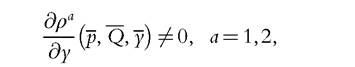
The specific nature of the identification result can be simply illustrated on a Cobb-Douglas example, as described later on. Before considering it, a few remarks are in order. First, the identification result stated in Theorem 1 is only local. This is important because additional constraints of a global nature (such as nonnegativity restric­tions on consumption), which are not considered in this result, typically provide addi­tional identification power; a precise illustration will be given below. Second, the result does not require distribution factors. Again, the latter would allow a stronger iden­tification result. Indeed, Chiappori and Ekeland show that, in the presence of distribution factors, the exclusivity requirement can be relaxed; one only needs either one excluded good (instead of two) or an assignable commodity.^[54] Third, identification requires the observation of the household demand as a function of prices and income; in particular, price variations are crucial. Although this fact is not surprising (even in standard consumer theory, preferences cannot be recovered from demand without price variations) it has important empirical applications, because data entailing significant (and credibly exoge­nous) price variations are not easy to find. However, recent approaches relax this require­ment by imposing additional structure on the decision process; they will be discussed below.

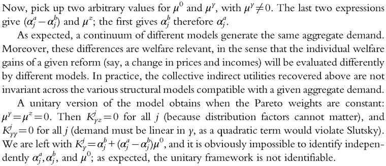
Fourth, the identification result above is only generic: it may fail to hold in particular cases, although such cases are not robust to “small variations.” Quite interestingly, one of the situations in which identification does not obtain is the unitary model. To see why, consider program (P) above, and assume that the Pareto weights μ^a are all constant. For

one thing, we are in a unitary context: the household maximizes the sum which is a price- and income-independent utility.

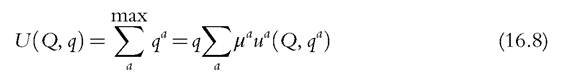
then the household maximizes U under the budget constraint. By standard integration, U can be recovered from the household demand. However, this is not sufficient to identify individual preferences: there exists a continuum of different sets of individual utilities that generate the same U by (16.8). The paradox here is that the unitary model, which used to be the dominant framework for empirical works on household behavior, belongs to the small (actually nongeneric) class of frameworks for which individual welfare cannot be identified from household demand.

Lastly, it is important to note that what is identified is the indirect collective utility of each member. From a welfare perspective, this is the only relevant concept, because it fully char­acterizes the utility reached by each agent. However, the inequality measures described above require more, namely, an assessment of the intrahousehold allocation of income. We now consider to what extent the latter can be recovered from the indirect collective utility.

16.5.1.2 Private Goods and the Sharing Rule

We start with the case in which all commodities are private. In that case, the various con­cepts (CSR, GSR, MMWI) coincide with the sharing rule, and the collective indirect utility takes the form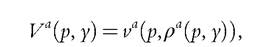

where, as above, v^a is a’s indirect utility and ρ is the sharing rule. Ifwe assume that the first (respectively the second) good is exclusively consumed by the second (first) agent, the col­lective indirect utility of each agent is identified (as always, up to some increasing transform).

16.5.1.2.1 Local Identification

A first result states that the sharing rule is not fully identified from the knowledge of the collective indirect utility, at least locally; identification only obtains up to an additive function of the prices of the nonexclusive goods.

Proposition 4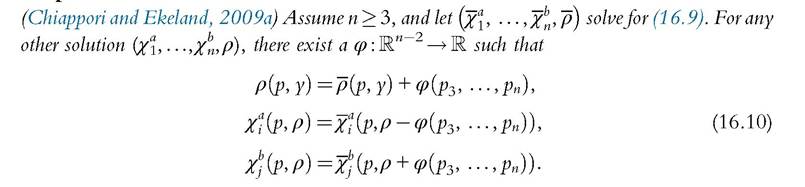

Moreover, overidentifying restrictions are generated.

The basic conclusion is that the sharing rule is identified up to an additive function, which cannot be pinned down unless either all commodities are assignable or individual preferences are known (for instance, from data on singles) or other (global) restrictions are used as described below. To see why, consider the simple case of three private commodities; two of these are exclusive (for members a and b, respectively), whereas the third is consumed by both. Individual consumptions of commodity 3 are not observed, and its price is taken as numeraire. In practice, we observe two demand functions q1 and q2 that satisfy

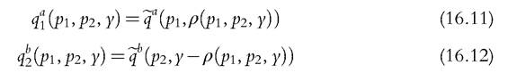
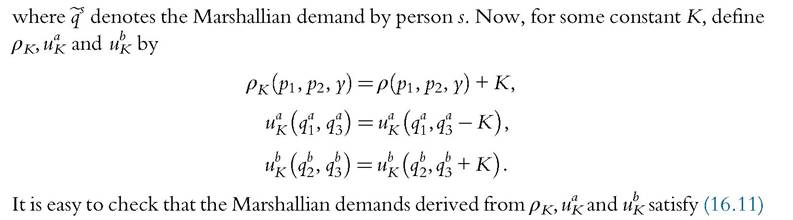
and (16.12). The intuition is illustrated in Figure 16.2 in the case of a. Switching from ρ and u^a to ρ_κ and uK does two things. First, the sharing rule and the intercept of the budget constraint are shifted downward by K. Second, all indifference curves are also shifted downward by the same amount. When only demand for commodity 1 (on the horizontal axis) is observable, these models are empirically indistinguishable. Lastly, with several, nonexclusive goods, this construct is still possible, and the constant may in addition vary with nonexclusive prices in an arbitrary way.

Two remarks can be made about this result. One is that the indetermination is not welfare relevant; one can easily check that the different solutions correspond to the same collective indirect utilities for each agent. This is the paradox evoked in introduction.

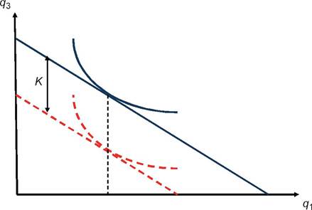
Figure 16.2 Welfare equivalence Ofalternative levels of the sharing rule.

16.5.1.2.2 Global Restrictions

The second remark is that the nonidentification result is only local. In particular, it disregards additional, global restrictions such as nonnegativity constraints. If these are added, then more can be identified. For instance, consider (16.10), and add the restric­tions that

which stems from nonnegativity of consumption at very low income levels. Then φ is exactly pinned down:

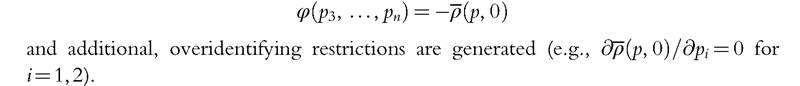
This result should be related to recent work on the estimation of the sharing rules based on a revealed preference approach (see, for instance, Cherchye et al., 2012). Because the revealed preference approach is global by nature, it can generate bounds on the sharing rule, which can actually be quite narrow. In all cases, the global restrictions are generated at one end of the distribution of expenditures, so their use for identifying the sharing rule outside this range should be submitted to the usual caution. Still, they tend to considerably reduce the scope of the nonidentification conclusion.

16.5.1.3 Public Goods Only

We now consider the opposite polar case, in which all commodities (but the exclusive ones) are public. That is, utilities are now of the form

Note that the exclusive commodities 1 and 2 can be considered as either public or private.

In that case, the collective indirect utility has a simple form, namely,

The crucial remark is that the demands for public goods (as functions of prices and total income) are empirically observed. An important consequence is that, in general, the knowledge of indirect collective utilities is equivalent to that of direct utilities. To see why, normalize y to be 1 (by homogeneity), and take a point at which theJacobian matrix D_p(Q₁, Q2, ■ ■ ■, Q_n) is of full rank. By the implicit function theorem, we can locally invert the function, thus defining P as a function of Q; but then,

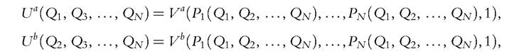
which proves identification. In addition, overidentifying restrictions are generated. In particular, we see that in this context Lindahl prices for all goods (therefore the MMWIs) are exactly identified. Somewhat paradoxically, the pure public good case appears to be the one in which identification is least problematic.

16.5.1.4 The General Case

Finally, the general case is a direct generalization of the two particular cases just described. The aforementioned exclusion restrictions guarantee identification of the collective indi­rect utility of each agent. Then the exact intrahousehold allocation is locally identified up to an additive function of the prices of the nonexclusive private goods. Moreover, global restrictions (e.g., nonnegativity) allow exact identification in general. The interested reader is referred to Chiappori and Ekeland (2009a,b) for detailed statements.

16.5.1.5 A Linear Expenditure System Example

The previous discussions can be illustrated on a simple example, borrowed from Chiappori and Ekeland (2009a). Consider individual preferences of the LES type: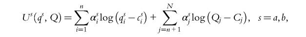

16.5.1.5.1 Household Demand

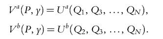
The couple solve the program

under the budget constraint. Individual demands for private goods are given by

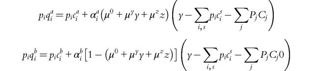
generating the aggregate demand

and for public goods

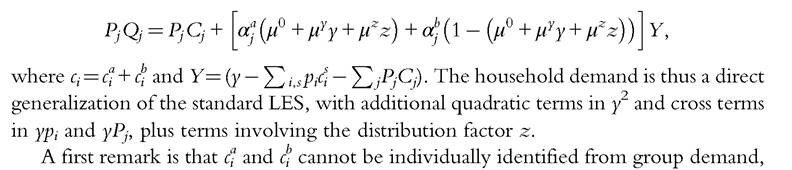
because the latter only involves their sum c_i. As a consequence, the various generalizations of the sharing rule will only be identified up to one additive constant, a result mentioned earlier. Also, the constant is welfare irrelevant; indeed, the collective indirect utilities of the wife and the husband are (up to an increasing transform)

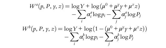
which does not depend on each c_i separately. Second, the form of aggregate demands is such that private and public goods have exactly the same structure. We, therefore, sim­plify our notations by defining

and similarly

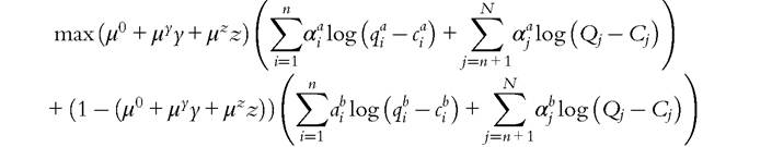
so that the group demand has the simple form

leading to collective indirect utilities of the form

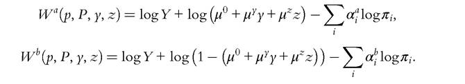
It is clear on this form that the distinction between private and public goods can be ignored. This illustrates an important remark: while the ex ante knowledge of the public versus the private nature of each good is necessary for the identifiability result to hold in general, for many parametric forms it is actually not needed.

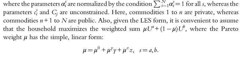
16.5.1.5.2 Identifiability: The General Case

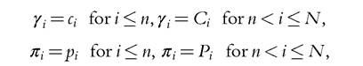
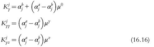
The question now is whether the empirical estimation of the form (16.14) allows us to recover the relevant parameters, namely, the α), the γ^t, and the μ^α. We start by rewriting (16.14) as

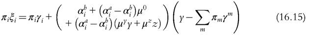
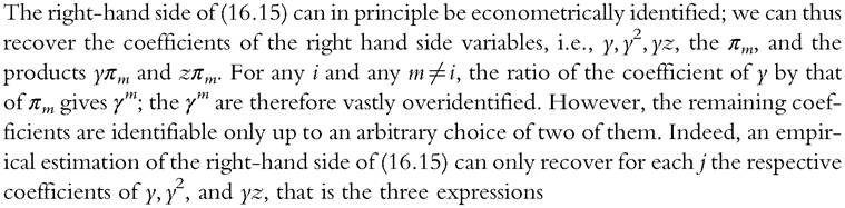
16.5.1.5.3 Identification Under Exclusion

We now show that in the nonunitary version of the collective framework, an exclusion assumption per member is sufficient to exactly recover all of the (welfare-relevant) coef­ficients. Assume that member a does not consume commodity 1, and member b does not consume commodity 2; that is, α^a₁ = α₂ = 0. Then equations (16.15) give

and

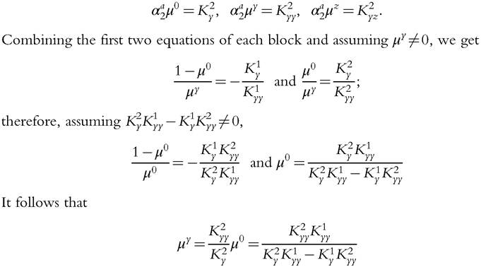
and all other coefficients can be computed as above. It follows that the collective indirect utility of each member can be exactly recovered, which allows for unambiguous welfare statements. As mentioned above, identifiability is only generic in the sense that it requires Clearly, the set of parameters values violating this condition is of zero

16.5.2 Comparing Different Family Sizes

A second approach enlarges the set of usable information by allowing comparisons between families of different compositions. A first idea is to assume some relationship between individual preferences when married and single. In that sense, the “pure” approach just described relies on an extreme version. This is because it does not postulate any link between utilities when married and single; hence, knowledge of an individual’s preferences when single brings no information about her tastes within the household. At the other extreme, some models assume that preferences are unaffected by marital status, at least ordinally. This means that if u^a_s(Q, q^a) denotes a’s utility when single, then her utility when married takes the form

where F is an increasing transform. Thus, marriage can directly affect a person’s utility level, but not the person’s marginal rates of substitution between various commodities. Note that if we assume preferences are unaffected by marital status, then the MMWI defined above has a natural interpretation; namely, it is the level of income that would be needed by the individual, if single, to reach the same utility level as what she currently gets within marriage. It must however be stressed that the assumption of constant pref­erences across marital status is not needed for the definition of the index, but only for this particular interpretation.

Various, intermediate approaches can be found in the literature. One, mostly used in a labor supply context, only assumes that some preference parameters are common to sin­gles and households, and can therefore be estimated separately on a sample of singles. In general, this is sufficient to identify (or calibrate) the remaining parameters (relevant for marriage-specific preferences and the Pareto weights) on observed labor supplies of men and women in a sample of couples. This approach has been adopted in a series of papers recently published in the Review of Economics of the Household (Bargain et al., 2006; Beninger et al., 2006; Myck et al., 2006; Vermeulen et al., 2006). For instance, consider a model of labor supply in a couple in which the utility of agent a takes the form

where L denotes leisure; note that this form is more general than the ones considered above, because it allows for (positive) externalities of leisure within the couple.¹⁴ The α and β parameters are assumed to be independent of marital status and are therefore iden­tified from a sample of singles; the γs and the Pareto weights are then calibrated from data on households.

An intermediate approach, that relies on the notion of domestic production, has recently been proposed by Browning et al. (2013). It posits that agents, when they get married, keep the same preferences but can access a different (and generally more pro­ductive) technology. That is, while the basic rates of substitution between consumed com­modities remains unaffected by marriage (or cohabitation), the relationship between purchases and consumptions is not; therefore, the structure of demand, including for exclusive commodities (consumed only by one member) is different from what it would be for singles. More generally, one can, following Dunbar et al. (2013), only assume that preferences are unaffected by family composition (e.g., that parents’ preferences regard­ing their own consumption does not depend on the number of children). These approaches are described in the next section.

14

Equivalently, this approach considers both leisures as public goods within the household.

16.5.3 Identifying from Market Equilibrium

Lastly, a series of recent contributions are aimed at taking to data the aforementioned equilibrium approaches. The basic, theoretical intuition is quite straightforward: the equilibrium conditions on the marriage market (with or without search frictions, but with intrahousehold transfers) either constrain or exactly pin down intrahousehold allo­cations. Several papers propose an empirical implementation of this idea. A first set of works only consider matching patterns; the marriage market equilibrium is then exclu­sively characterized by a matrix of intermarriages between various categories, which can be defined by age, education, income, or any combination of these. On the matching front, following the initial contribution by Choo and Siow (2006), Chiappori et al. (2011) have shown how a structural, parametric model can be (over)identified from such patterns, under the assumption that, while the surplus generated by marriage may (and does) vary over time, its supermodularity (which drives the extent of assortative matching in the population) is constant.^[55] According to their estimate, while the gains from mar­riage have globally decreased over the last decades, the decline has been much smaller for educated couples. Moreover, the share of household resources received has increased for college-educated wives, resulting in a strong increase in their “marital college premium” (defined as the additional gain provided by a university education on the marriage mar­ket). This is compatible with the theoretical analysis of Chiappori et al. (2009), who argued that the asymmetry between male and female marital college premiums could explain (at least in part) the higher demand for university training by women. Alterna­tively, Jacquemet and Robin (2011) and Gousse (2013) analyze marital patterns from a search perspective.

A clear limitation of these approaches is that the sole observation of marital patterns conveys only limited information on the form of the marital surplus (therefore on dis­tribution). For instance, knowing that matching is assortative tells us only that the surplus is supermodular. The previous approaches, therefore, must rely on strong and largely untestable assumptions on the precise form of the heterogeneity distribution across cou­ples. Adding information on the total surplus would greatly enhance the identification power of these models. But such information is precisely what collective models can pro­vide based on observed behavior. The intuition, here, is that the observation of, say, labor supply patterns of married couples (which reflects intrahousehold transfers), together with that of marital patterns, should allow us to fully identify a general matching model in a very robust way. This line of research is pursued, in a series of paper, by Chiappori et al. (2014).

16.6.