THE DETERMINANTS OF INTRAHOUSEHOLD ALLOCATION
The second task assigned to theory is to explain the allocation of powers, hence of resources, within the household. As such, it must address issues related to household
formation and dissolution, as well as the interaction between the household and its environment, that is, which external factors may impact the intrahousehold decision process.
In what follows, we concentrate on two types of approaches, respectively based on cooperative bargaining and matching or search theory. In a sense, this distinction reflects the classic dichotomy between partial and general equilibrium. Bargaining models analyze, for a given household, how the particular situation of each member may affect the household decision; much emphasis is put on individual “threat points,” generally considered as exogenous. Matching and search models, on the other hand, describe a global equilibrium on the “market for marriage” as a whole. Although the decision process may in some cases entail bargaining (in search models, or in matching with a finite set of agents), the crucial distinction is that the threat points are now endogenous—their determination is part of the equilibrium conditions.16.4.1 Bargaining Models
Any bargaining model requires a specific setting: In addition to the framework described above (K agents, with specific utility functions), one has to define a threat point T for each individual a. Intuitively, a person’s threat point describes the utility level this person could reach in the absence of an agreement with the partner. Typically, bargaining models assume that the outcome of the decision process is Pareto efficient and individually rational, in the sense that individuals never receive less than their threat point. Bargaining theory is used to determine how the threat points influence the location of the chosen point on the Pareto frontier.
Clearly, if the point T = (T1,..., Tk) is outside of the Pareto set, then no agreement can be reached, because at least one member would lose by agreeing. However, if T belongs to the interior of the Pareto set so that all agents can gain from the relationship, the model picks a particular point on the Pareto utility frontier. Note that the crucial role played by threat points—a common feature of all bargaining models—has a very natural interpretation in terms of distribution factors. Indeed, any variable that is relevant for threat points only is a potential distribution factor. For example, the nature of divorce settlements, the generosity of single-parent benefits, or the probability of remarriage do not directly change a household’s budget constraint (as long as it does not dissolve), but may affect the respective threat points of individuals within it. Then bargaining theory implies that they will influence the intrahousehold distribution of power in households and, ultimately, household behavior. Equivalently, one could say that these variables are distribution factors that affect the Pareto weights.In practice, models based on bargaining must make a number of basic choices. One is the bargaining concept to be used. Whereas most studies refer to Nash bargaining, some either adopt Kalai-Smorodinski or refer to a noncooperative bargaining model. Second, one must choose a relevant threat point. This part is crucial; indeed, a result due to Chiappori et al. (2012) states that any Pareto efficient allocation can be derived as the Nash bargaining solution for an ad hoc definition of the threat points. Hence any additional information provided by the bargaining concepts (besides the sole efficiency assumption) must come from specific hypotheses on the threat points, that is, on what is meant by the sentence “no agreement is reached.” Several ideas have been used in the literature. One is to refer to divorce as the “no agreement” situation.
Then the threat point is defined as the maximum utility a person could reach after divorce. Such an idea seems well adapted when one is interested, say, in the effects of laws governing divorce on intrahousehold allocation. It is probably less natural when minor decisions are at stake: Choosing who will walk the dog, for example, is unlikely to involve threats of divorce.[53] Another interesting illustration would concern public policies that affect single parents, or the guaranteed employment programs that exist in some Indian states. Haddad and Kanbur (1992) convincingly argue that the main impact of the program was to change the opportunities available to the wife outside of marriage.A second idea relies on the presence of public goods and the fact that noncooperative behavior typically leads to inefficient outcomes. The idea, then, is to take the noncooperative outcome as the threat point: In the absence of an agreement, both members provide the public good(s) egotistically, not taking into account the impact of their decision on the other member’s welfare. This version captures the idea that the person who would suffer more from this lack of cooperation (the person who has the higher valuation for the public good) is likely to be more willing to compromise in order to reach an agreement. A variant, proposed by Lundberg and Pollak (1993), is based on the notion of “separate spheres.” The idea is that each partner is assigned a set of public goods to which they alone can contribute; this is their “sphere” of responsibility or expertise. These spheres are determined by social norms. Then the threats consist of continued marriage in which the partners act noncooperatively and each chooses independently the level of public goods under their domain.
Finally, it must be reminded that assumptions on threat points tend to be strong, not grounded on strong theoretical arguments, and often not independently testable. This suggests that models based on bargaining should be used parsimoniously and with care.
16.4.2 Equilibrium Models
Alternatively, one can consider the “market for marriage” as a whole from a general perspective.
Two types of models can be found in the literature, that make opposite assumptions on the role of frictions in the matching game. Specifically, models based on matching (with transferable or imperfectly transferable utility, TU and ITU, respectively) assume away frictions and consider perfectly smooth markets, while models based on search emphasize the importance of frictions in the emergence of marital patterns. While matching and search-based approaches use different technologies, their scope and outcomes are largely similar for what we are concerned with here. In what follows, for the sake of brevity, we therefore concentrate on matching models. Moreover, we only discuss models based on TU. The nontransferable utility framework, which assumes away any transfer between members, is not relevant here. And although more general approaches based on ITU have recently been developed (see Chiappori, 2012), the distinction between TU and ITU can basically be disregarded for our current discussion.Consider the two populations of men and women: Each individual is defined by a vector of characteristics, denoted x 2 X for women and y 2 Y for men. Both sets are endowed with a finite measure, denoted μx and μγ, respectively. When matched, Mrs. x and Mr. y jointly generate a surplus s(x, y), which can be derived from a more structural framework (e.g., a collective model). A matching is defined by (i) a measure μ on the set X? Y, the marginals of which coincide with μx and μγ, and (ii) two functions u(x) and v(y) such that u(x) + v(y) = s(x, y) on the support of μ. Intuitively, the measure μ defines who marries whom, whereas the functions determine how the surplus is divided within couples who are matched with positive probability: She gets u(x), he gets v(y). A matching is stable if (i) no married person would prefer being single and (ii) no pair of currently unmarried persons would both prefer forming a new couple.
Technically, this is equivalent to
The functions u(x) and v(y) are crucial, inasmuch as they fully determine the intrahousehold inequality. The key feature of matching models is that these functions are endogenous. They are determined (or constrained) as part of the equilibrium, and depend on the whole matching game structure; in particular, the allocation within any given couple depends on the entire distribution of characteristics in the two populations. In that sense, the model does provide an endogenous determination of intrahousehold inequality. Note, however, that in this abstract presentation, their exact interpretation is undetermined; depending on the framework, u(x) can be a monetary amount, the consumption of some commodity or the utility generated by the consumption of bundles of private and public commodities. For instance, the simple framework used by Chiappori and Weiss (2007) consider an economy with two commodities, one private and one public within the household, and agents with Cobb-Douglas preferences ua = qaQ; x and y are onedimensional and denote male and female income. In this TU framework, any efficient allocation maximizes the sum of utilities; that is, a (x, y) couple solves

and the surplus s(x, y) is the value of this program, namely (x + y)2∕4. Here, u(x) and v(y) are utilities, although there exists a one-to-one correspondence between utilities and 
From a mathematical point of view, a basic result states that, if a matching is stable, then the corresponding measure maximizes total surplus over the set of measures whose marginals coincide with μx and μγ. That is, the measure μ must solve
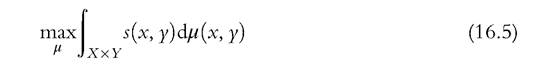
under the marginal conditions.
This maximization problem is linear in its unknown μ. Therefore, it admits a dual, which can be written as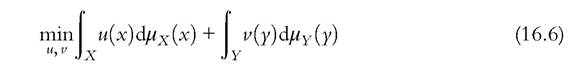
under the constraints

Here, functions u and v are the dual variables of the program. But, crucially, they can be interpreted as describing the utility reached by each individual at optimal matching. In particular, they define the allocation of surplus between (matched) spouses. Note that conditions of the dual program (16.7) are exactly the stability conditions (16.3).
From the standard duality results, a solution to the dual exists if and only if the primal has a solution, and the values are then the same. It follows that the existence of a stable match (that is, of functions u and v satisfying (16.3)) boils down to the existence ofa solution to the linear maximization problem (16.5). This allows us to establish existence under very general conditions; see, for instance, Chiappori et al. (2010).
Regarding uniqueness, if the sets X and Y are finite, then the u s and vs are not pinned down, although the equilibrium conditions generate constraints. However, with continuous, atomless populations, the functions are in general fully determined by the equilibrium conditions. The intuition is straightforward: in the continuous case, each individual has almost perfect substitutes, and (local) competition determines exactly the surplus sharing that must exist at equilibrium. Finally, stochastic versions of these models can be considered, in which some of the individual characteristics are unobserved (to the econometrician); see, for instance, the recent survey by Chiappori and Salanie (2014).
16.5.