MODELING HOUSEHOLD BEHAVIOR: THE COLLECTIVE MODEL
16.3.1 Private Goods Only: The Sharing Rule
We first consider a special case in which all commodities are privately consumed. Then the household can be considered as a small economy without externalities or public goods.
From the second welfare theorem, any Pareto efficient allocation can be decentralized by adequate transfers; formally, we have the following result: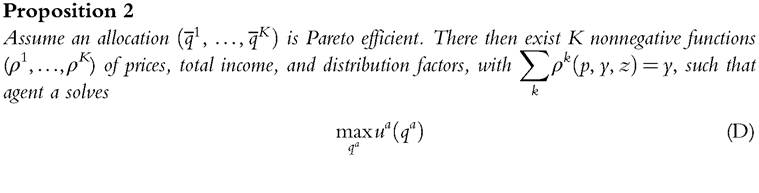
[1] In practice, distribution factors must also be uncorrelated with unobserved components of preferences, which, in the case of individual incomes, can generate subtle exogeneity problems. See Browning et al. (2014) for a detailed discussion.
under the budget constraint
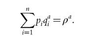

In words, in a private-goods setting, any efficient decision can be described as a two- stage process. In the first stage, agents jointly decide on the allocation ofhousehold aggregate income y between agents (and agent a gets ρa); in the second stage, agents freely spend the shares they have received. The decision process (bargaining, for instance) takes place in the first stage; its outcome is given by the functions (ρ1,..., ρκ), which are called the sharing rule of the household. From a welfare perspective, there exists a one-to-one, increasing correspondence between Pareto weights and the sharing rule, at least when the Pareto set is strictly convex: when prices and incomes are constant, increasing the weight of one individual (keeping the other weights unchanged) always results in a larger share for that individual. The converse is also true.
Finally, the collective, indirect utility takes a simple form, namely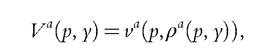
where va is the standard, indirect utility of agent a. We therefore have the following result:
Proposition 3
When all commodities are privately consumed, then for any given price vector there exists a one-to- one correspondence between the sharing rule and the indirect utility.
In particular, a member’s collective indirect utility can be directly computed from the knowledge of that person’s preferences and sharing rule; given the preferences, the sharing rule is a sufficient statistic for the entire decision process.
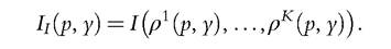
Regarding the issue of intrahousehold inequality, the key remark is that the sharing rule contains all the information required: Because all agents face the same prices, the sharing rule fully summarizes intrahousehold allocation of resources. As such, it is directly relevant for intrahousehold inequality. Specifically, let I(y1,...,yn) be some inequality index (as a function of individual incomes). Then the intrahousehold index of inequality is
16.3.2 Public and Private Commodities
Convenient as the previous notion may be, it still relies on a strong assumption, namely that all commodities are privately consumed. Relaxing this assumption is obviously necessary, if only because the existence of public consumption is one of the motives of household formation.
Different notions have been considered in the literature. The notion of conditional sharing rule (CSR), initially introduced by Blundell et al. (2005), refers to a two-stage process, whereby in stage one the household decides the consumption of public goods and the distribution of remaining income between members. In stage two all members spend their allotted amount on private consumptions to maximize individual utility conditional on the level of public consumption decided in stage one.
As before, any efficient decision can be represented as stemming from a two-stage process of that type. The converse, however, is not true: for any given level of public consumptions, almost all CSRs lead to inefficient allocations. Moreover, the monotonic relationship between sharing rule and Pareto weights is lost. In particular, increasing a’s weight does not necessarily result in a larger value for a’s CSR; the intuition being that more weight to one agent may result in a different allocation of public expenditures, which may or may not result in an increase in the agent’s private consumption. Lastly, and more importantly for our purpose, the CSR may give a biased estimate of intrahousehold inequality, because it simply disregards public consumption. That this pattern could be problematic is easy to see. Assume that one spouse (say the wife) cares a lot for a public good, whereas her husband cares very little. If the structure of household demand entails a significant fraction of expenditures being devoted to that public good, one can expect this pattern to have an impact on any inequality measure within the household. Disregarding public consumption altogether is therefore not an adequate approach.A second approach relies on an old result in public economics, stating that in the presence of public goods, any efficient allocation can be decentralized using personal (or Lindahl) prices for the public good. This result establishes a nice duality between private and public goods: for the former, agents face identical prices and purchase different quantities (the sum of which is the household’s aggregate demand), whereas for the latter the quantity is the same for all but prices are individual specific (and add up to market prices). Again, the household behaves as if it was using a two-stage process. In stage one the household chooses a vector of individual prices for the public goods and an allocation of total income between members; in stage two members all spend their income on private and public consumptions under a budget constraint entailing their Lindahl prices.
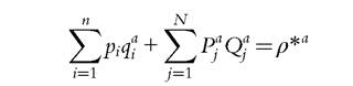
Formally, member a solves
under the budget constraint
See Chiappori and Ekeland (2009b) for a general presentation. For applications, see for instance Donni (2009) and Cherchye et al. (2007, 2009) for a revealed preferences perspective.
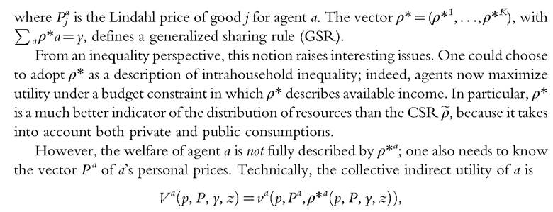
which depends on both ρ*a and Pa. This implies that the sole knowledge of the GSR is not sufficient to recover the welfare level reached by a given agent, even if her preferences are known; indeed, one also needs to know the prices, which depend on all preferences. In particular, we believe that the level of inequality within the household cannot be analyzed from the sole knowledge of the GSR. Agents now face different personal prices, and this should be taken into account. Of course, this conclusion was expected; it simply reflects a basic but crucial insight, namely that if agents “care differently” about the public goods (as indicated by personal prices, which reflect individual marginal willingness to pay), then variations in the quantity of these public goods have an impact on intrahousehold inequality.
Finally, Chiappori and Meghir (2014) have recently proposed the concept of Money Metric Welfare Index (MMWI). Formally, the MMWI of agent a, ma(p, P, y, z), is defined by

In words, ma is the monetary amount that agent a would need to reach the utility-level Va(p, P, y), if she was to pay the full price of each public good (i.e., if she faced the price vector P instead of the personalized prices Pa). The basic intuition is simple enough. The index is defined as the monetary amount that would be needed to reach the same utility level at some reference prices.
A natural benchmark is to use the current market price for all goods, private and public. In particular, there exists a direct relationship between the MMWI and the standard notion of equivalent income; although to the best of our9
See for instance Fleurbaey et al. (2014).
knowledge, equivalent income has mostly been applied so far to private goods.10 Both approaches rely on the notion that referring to a common price vector can facilitate interpersonal comparisons of welfare.
Unlike the GSR, the MMWI fully characterizes the utility level reached by the agent. That is, knowing an agent’s preferences, there is a one-to-one relationship between her utility and her MMWI, and this relationship does not depend on the partner’s characteristics. In the pure private goods case, the MMWI coincides with the sharing rule; it generalizes this notion to a general setting without losing its main advantage, namely the one-to-one relationship with welfare. Finally, it can readily be extended to allow for labor supply and domestic production; the reader is referred to Chiappori and Meghir (2014) for a detailed presentation.
16.3.3 An Example
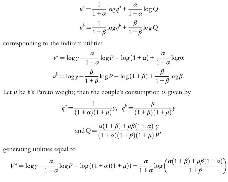
The previous concepts can be illustrated on a very simple example, borrowed from Chiappori and Meghir (2014). Assume two agents a and b, two commodities—one private q, one public Q—and Cobb-Douglas preferences:
10 See, however, Hammond (1995) and Fleurbaey and Gaulier (2009).
'~-i
Assume now that μ = 1, but agents have different preferences for the public good. For instance, α = 2 while β = 0.5, implying that the wife (or husband) puts two-thirds of the weight on the public (private) consumption. In this setting, we can analyze intrahousehold inequality using three possible indicators.
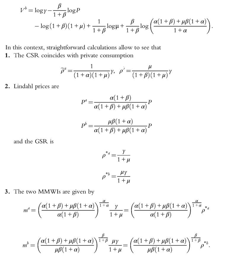
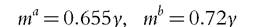
1. If we concentrate on private consumption (or equivalently on the CSR), we find that
and we conclude that member b is much better off than a.
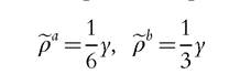
2. This conclusion is clearly unsatisfactory, because it disregards the fact that half the budget is spent on the public good, which benefits a more than b. Indeed, the GSR is
and we conclude that for this indicator, the household is perfectly equal: the benefits of public expenditures exactly compensate differences in private consumptions.
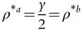
3. The later conclusion is, however, too optimistic, as it omits the fact that a “pays” twice as much for the public good than b does (here,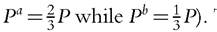 Taking
this last aspect into account, the respective MMWIs are
Again, b is better off than a (although by much less than with the first measure). In addition, one may note that
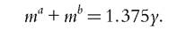
Individual MMWIs add up to more than total income, reflecting the gain generated by the publicness of one commodity.
16.3.4 Domestic Production
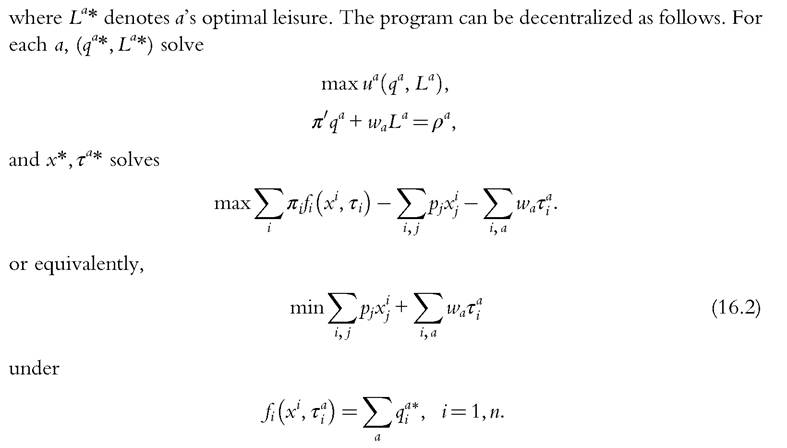
Finally, the previous analysis can readily be extended to domestic production. Here, we only consider the case where all commodities are privately consumed; for a more general presentation along similar lines, the reader is referred to Chiappori and Meghir (2014). The household production technology is thus described by a production function that gives the possible vector of outputs q =f(x, τ), that can be produced given a vector of market purchases x and the time τ = (τa, a = 1, K) spent in household production by each of the members.
We first disregard the time spent by each member on domestic production. This setting is thus identical to the general model of household production of Browning et al. (2013).11 Pareto efficiency translates into the program
where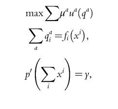
11 For empirical applications, these authors use a linear technology a la Barten.
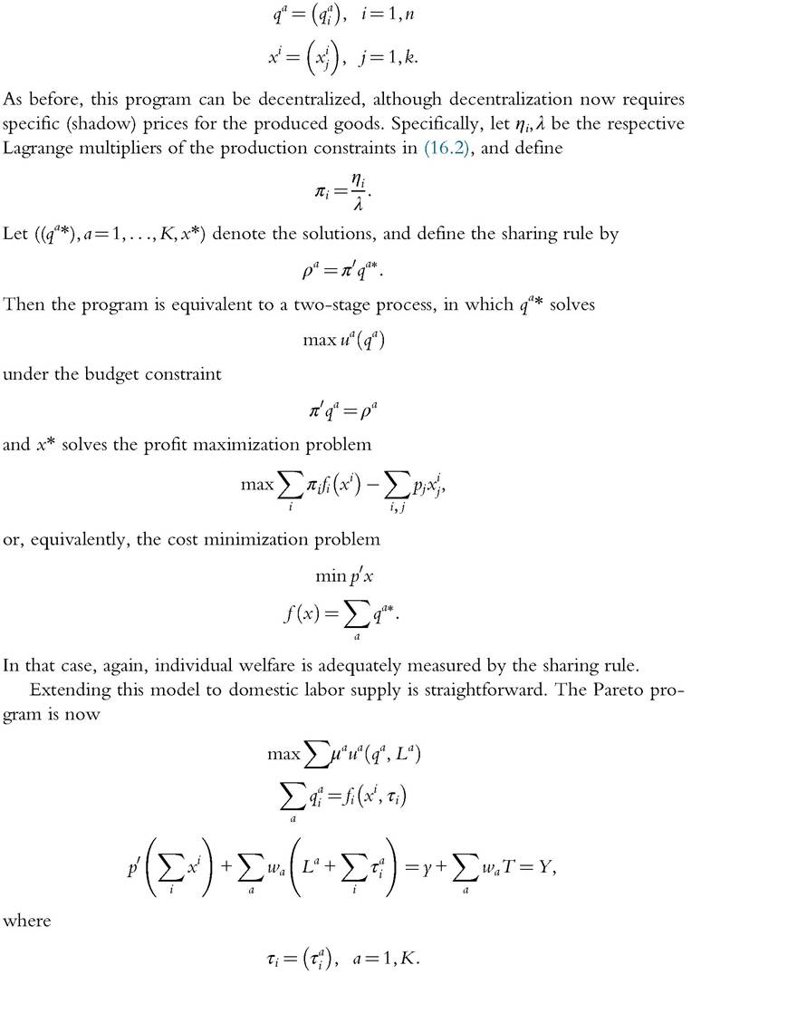
Prices for internally produced goods are defined as before. The sharing rule is now
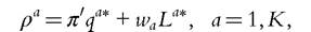
In practice, several variants of this basic framework can be considered, depending on whether the internally produced goods are marketable, and whether market labor supplies are available via an interior or a corner solution. These technical issues are not without importance. For instance, a standard issue in family economics is whether a change in the respective powers of the various members has an impact on the intrahousehold allocation of domestic work. In the model just described, if the produced commodities are marketable and all individuals work on the market, then the πs and the ws must coincide with market prices and wages; they are therefore exogenous, and individual, domestic labor supplies are fully defined by the program (16.2), which does not depend on Pareto weights. We conclude that, in that case, powers have no impact on domestic work, which is fully determined by efficiency considerations. Clearly, this argument must be modified when either the πs or the ws are endogenous (as will be the case if, respectively, the commodity is not marketable or a person does not participate in the labor market). The reader is referred to Browning et al. (2014) for a precise discussion, as well as to the Chapter 12 in this handbook.
16.4.