THE COLLECTIVE MODEL: CONCEPTS, DEFINITIONS, AND AXIOMS

In what follows, we consider a K-person household that can consume several commod­ities; these may include standard consumption goods and services, but also leisure, future or contingent goods, and the like.

⁴ See Browning et al. (2014).

⁵ Browning et al. (2008) and Lechene and Preston (2011) provide a set of necessary conditions for nonco­operative models. However, whether these conditions are sufficient is not known; moreover, no general identification result has been derived so far.

Lastly, a particular but widely used version of caring is egotistic preferences, whereby members only care about their own (private and public) consumption;then individual preferences can be represented by felicities (i.e., utilities of the formNote that

such egotistic preferences for consumption do not exclude noneconomic aspects, such as love, companionship, or others. That is, a person’s utility may be affected by the presence of other persons, but not by their consumption. Technically, the “true” preferences are of the formwhere F^a may depend on marital status and on the spouse’s char­

acteristics. Note that the F^αs will typically play a crucial role in the decision to marry and in the choice of a partner. However, it is irrelevant for the characterization of married individuals’ preferences over consumption bundles.

Efficiency has a simple translation; namely, the household behaves as if it was max­imizing a weighted sum of utilities of its members. Technically, the program is thus (assuming egotistic preferences):

under the budget constraint: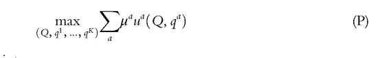

Throughout the chapter, we assume, for convenience, that utility functions u^a(∙), a = 1, K are continuously differentiable and strictly quasi-concave.

very special role, because any allocation that is efficient for caring preferences must be efficient for the underlying, egotistic felicities, as stated by the following result:

Proposition 1

Proof

The converse is not true, because a very unequal solution to (P) may fail to be Pareto efficient for caring preferences: transferring resources from well-endowed but caring individuals to the poorly endowed ones may be Pareto improving. Still, any property of the solutions to a program of the form (P) must be satisfied by any Pareto-efficient allocation with caring preferences.

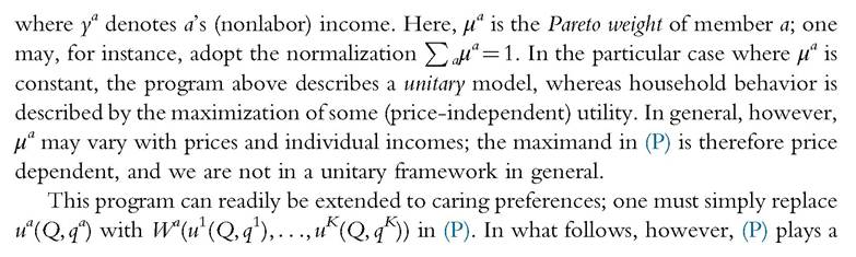
A major advantage of the formulation (P) is that the Pareto weights have a natural interpretation in terms of respective decision powers. The notion of “power” in house­holds may be difficult to define formally, even in a simplified framework such as ours. Still, it seems natural to expect that when two people bargain, a person’s gain increases with the person’s power. This somewhat hazy notion is captured very effectively by the Pareto weights. Clearly, if μ^a in (P) is zero, then a has no say on the final allocation, whereas if μ^α is large, then a effectively gets her way.

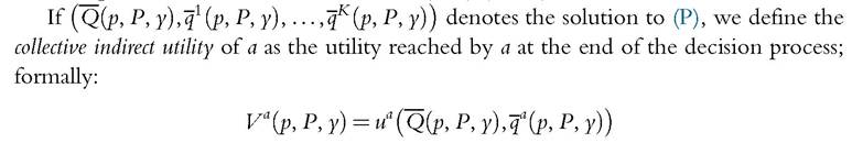
Note that, unlike the unitary setting, in the collective framework a member’s collective indirect utility depends not only on the member’s preferences but also on the decision process (hence the adjective “collective”). This notion is crucial for welfare analysis, as we shall see below.

Finally, an important concept is the notion of “distribution factors.” A distribution factor is any variable that (i) does not affect preferences or the budget constraint, but (ii) may influence the decision process, therefore the Pareto weights. Think, for instance, of a bargaining model in which the agents’ respective threat points may vary. A change in the threat point of one member will typically influence the outcome of the bargaining process, even if the household’s budget constraint is unaffected. In particular, several tests

of household behavior consider the income pooling property. The basic intuition is straightforward: in a unitary framework, whereby households behave like single decision makers (and maximize a unique, income-independent utility), only total household income should matter. Individual contributions to total income have no influence on behavior: they are pooled in the right-hand side of the household’s budget constraint. For instance, paying a benefit to the wife rather than to the husband cannot possibly impact the household’s demand. As we will see later, this property has been repeatedly rejected by the data. The most natural interpretation for such rejections (although not the only one) is that individual incomes may impact the decision process (in addition to their 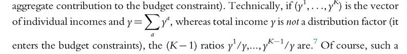setting by no means implies that each individual consumes exactly his or her income.

In what follows, the vector of distribution factors will be denoted z = (z₁,..., z_S); Pareto weights and collective indirect utilities, therefore, have the general form

16.3.