Identification of the Poor: The Dual-Cutoff Approach

Poverty measurement requires an identification function, which determines whether each person is to be considered poor. The unidimensional form of identification, discussed in section 2.1.1, entails a host of assumptions that restrict its applicability in practice and its desirability in principle.^[162] From the perspective of the capability approach, a key conceptual drawback of viewing multidimensional poverty through a unidimensional lens is the loss of information on dimension-specific shortfalls; indeed, aggregation before identification converts dimensional achievements into one another without regard to dimension-specific cutoffs.

In the multidimensional measurement setting, where there are multiple variables, identification is a substantially more challenging exercise. As explained in section 2.2.2, a variety of methods can be used for identification in multidimensional poverty measurement. Here we follow a censored achievement approach. This approach first requires determining who is deprived in each dimension by comparing the person's achievement against the corresponding deprivation cutoff and thus considering only deprived achievements (and ignoring—or censoring—achievements above the depriva­tion cutoff) for the identification of the poor. One prominent method used within the censored achievement approach is the counting approach, which is precisely the identification approach followed in the AF methodology, among others (Chapter 4).

As we have seen, a counting approach first identifies whether a person is deprived or not in each dimension and then identifies a person as poor according to the number (count) of deprivations she experiences.

Second, as a consequence of using a dual-cutoff approach, the AF methodology considers the joint distribution of deprivations at the identification step and not just at the aggregation step, as previous methodologies did (almost all non-counting methodologies used the union criterion). Third, the AF methodology has integrated the counting approach to identification with an aggregation methodology that extends the unidimensional FGT measures, overcoming the limitations of the headcount ratio (which most counting methods used) yet allowing intuitive interpretations.^[163]

Thus the AF methodology draws together the counting traditions—well-known for their practicality and policy appeal—and the widely used FGT class of axiomatic measures in order to assess multidimensional poverty, and stands on the shoulders of both traditions.

5.2.1 THE DEPRIVATION CUTOFFS: IDENTIFYING DEPRIVATIONS AND OBTAINING DEPRIVATION SCORES

Bourguignon and Chakravarty (2003) contend that ‘a multidimensional approach to poverty defines poverty as a shortfall from a threshold on each dimension of an individual's wellbeing'.^[164] Following them and the plethora of counting methods reviewed in Chapter 4, the AF measures use a deprivation cutoff for each dimension, defined and applied as described in this section.

As introduced in section 2.2, the base information in multidimensional poverty measurement is typically represented by an n ? d dimensional achievement matrix X, where x_ij is the achievement of person i in dimension j. For simplicity, as done in section 2.2, it is assumed that achievements can be represented by non-negative real numbers (i.e. x_ij ∈ R₊) and that higher achievements are preferred to lower ones.

For each dimension j, a threshold Zj is defined as the minimum achievement required in order to be non-deprived. This threshold is called a deprivation cutoff. Deprivation cutoffs are collected in the d-dimensional vector z = (z₁,...,z_d). Given each person’s achievement in each dimension x_ij, if the i^th person’s achievement level in a given dimension j falls short of the respective deprivation cutoff Zj, the person is said to be deprived in that dimension (that is, if x_ij < Zj). If the person’s level is at least as great as the deprivation cutoff, the person is not deprived in that dimension.

As Chapter 2 introduced, from the achievement matrix X and the vector of deprivation cutoffs z, one can obtain a deprivation matrix g⁰ such that g0 = 1 whenever x_ij < Zj and go = 0, otherwise, for all j = 1,..., d and for all i = 1,..., n. In other words, if person i is deprived in dimension j, then the person is assigned a deprivation status of 1, and 0 otherwise. The matrix g⁰ summarizes the deprivation status of all people in all dimensions of matrix X. The vector g_i⁰ summarizes the deprivation statuses of person i in all dimensions, and the vector g0 summarizes the deprivation statuses of all persons in dimension j.

The deprivation in each of the d dimensions may not have the same relative importance. Thus, a vector w = (w₁,..., w_d) of weights or deprivation values is used to indicate the relative importance of a deprivation in each dimension.

Intricate weighting systems create challenges in interpretation, so it can be useful to choose the dimensions such that the natural weights among them are roughly equal or else to group dimensions into categories that have roughly equal weights (Atkinson 2003). The deprivation values affect identification because they determine the minimum combinations of deprivations that will identify a person as being poor. They also affect aggregation by altering the relative contributions of deprivations to overall poverty (for more on weights see Chapter 6). Yet, importantly, the deprivation values do not function as weights that govern trade-offs between dimensions for every possible combination of ratio-scale achievement levels, as they do in a traditional composite index. Because each deprivation status takes binary value, the role of deprivation values differs from the role of weights in traditional composite indices.

Based on the deprivation profile, each person is assigned a deprivation score that reflects the breadth of each person’s deprivations across all dimensions. The deprivation score of each person is the sum of her weighted deprivations. Formally, the deprivation score is given by c_i = ∑' ₁ Wjg0j = ∑' ₁ g0j. The score increases as the number of deprivations a person experiences increases, and reaches its maximum when the person is deprived in all dimensions. A person who is not deprived in any dimension has a deprivation score equal to 0. We denote the deprivation score of person i by c_i and the vector of deprivation scores for all persons by c = (c₁,..., c_n).

5.2.2 ALTERNATIVE NOTATION AND PRESENTATION

Distinct notational presentations can be employed for the weights, deprivation scores, deprivation score vector, poverty cutoff, poverty measures, and partial indices. Sub­stantively, alternative presentations are identical in that they each identify precisely the same persons as poor and generate the same poverty measure value and identical partial indices. What differ are the numerical values of weights, deprivation scores, and poverty cutoff. For didactic purposes we explain the main options so as to avoid confusion among researchers using different notational conventions.

Alternative notations arise from two decisions. The first decision is whether to define weights that sum to one, i.e. ∑_j w_j = 1, or whether weights sum to the number of dimensions under consideration, ∑λ w_j = d. We refer to the first as normalized weights and to the second as non-normalized or numbered weights. The normalized weight of a dimension reflects the share (or percentage) of total weight given to a particular dimension. The deprivation score then shows the percentage of weighted dimensions in which a person is deprived and lies between 0 and 1. In the numbered case, deprivation scores range between 0 and d. If person i is deprived in all dimensions, then c_i = d. Depending on the weighting structure, one of these options may be more intuitive than the other. For example, if dimensions are equally weighted, the deprivation count vector shows the number of dimensions in which each person is deprived. Thus, while in the normalized case one may state that a person is deprived in 43% of the weighted dimensions, in the non-normalized case one states that a person is deprived in three out of seven dimensions, which is more intuitive. However, if dimensions are not equally weighted, normalized weights maybe more intuitive. Suppose there are seven dimensions and a person is deprived in two dimensions having weights of 25% and 10%, respectively.

The second decision is whether to express the formulas using the deprivation matrix g⁰ and the weighting vector w in an explicitly separate way, or whether to express them in terms of a weighted deprivation matrix denoted by g⁰ such that g0 = w_j if g⁰ = 1 and g⁰ = 0 if g⁰ = 0. These two decisions lead to four possible—but totally equivalent—notations, as detailed in Box 5.7. This chapter, and most of this book, uses normalized weights and expresses formulas using the deprivation matrix and the weight vector. We refer to this as Method I. Method II uses normalized weights with the weighted deprivation matrix. Method III uses non-normalized weights and expresses formulas using the deprivation matrix and the weight vector. Methods II and III are not further discussed in this chapter, but all the formulas are stated in Box 5.7. Finally, Method IV uses non-normalized weights and expresses the formulas using the weighted deprivation matrix, aligned with the notation used in Alkire and Foster (2011a), which is presented in Box 5.3, Box 5.6, and Box 5.7. What is particularly elegant about Method IV is that the AF measures can be expressed as the mean of the relevant censored deprivation matrix, as we shall elaborate subsequently.

5.2.3 THE SECOND CUTOFF: IDENTIFYING THE POOR

In addition to the deprivation cutoffs Zj, the AF methodology uses a second cutoff or threshold to identify the multidimensionally poor. This is called the poverty cutoff and is denoted by k. The poverty cutoff is the minimum deprivation score a person needs to exhibit in order to be identified as poor. This poverty cutoff is implemented using an identification function ρ_k, which depends upon each person's achievement vector x_i., the deprivation cutoff vector z, the weight vector w, and the poverty cutoff k. If the person is poor, the identification function takes on a value of 1; if the person is not poor, the iden­tification function has a value of 0. Notationally, the identification function is defined as ρ_k(x_i ∙; z) = 1 if c_i ≥ k and ρ_k (x_i.∙,z) = 0 otherwise. In other words, ρ_k identifies person i as poor when his or her deprivation score is at least k; if the deprivation score falls below the cutoff k, then person i is not poor according to ρ_k. Since ρ_k is dependent on both the set of within-dimension deprivation cutoffs z and the across-dimension cutoff k, ρ_k is referred to as the dual-cutoff method of identification, or sometimes as the ‘intermediary' method.

Within the counting approach to identification, the most commonly used multidi­mensional identification strategy is the union criterion.^[165] Most of the poverty indices discussed in Chapter 3 use the union criterion, by which a person i is identified as multidimensionally poor if she is deprived in at least one dimension (c_i > 0). At the other extreme, another identification criterion is the intersection criterion, which identifies person i as being poor only if she is deprived in all dimensions (c_i = 1). Both these approaches have the advantage of identifying the same persons as being poor regardless of the relative weights set on the dimensions. But the identification of who is poor in each case is exceedingly sensitive to the choice of dimensions. Also these strategies can be too imprecise for policy: in many applications, a union identification identifies a very large proportion of the population as poor, whereas an intersection approach identifies a vanishingly small number of people as poor. A natural middle-ground alternative is to use an intermediate cutoff level for c_i that lies somewhere between the two extremes of union and intersection.

The AF dual-cutoff identification strategy provides an overarching framework that includes the two extremes of union and intersection criteria and also the range of intermediate possibilities.^[166] Notice that ρ_k includes the union and intersection methods as special cases. In the case of union, the poverty cutoff is less than or equal to the dimension with the lowest weight: 0 < k ≤ min {w₁,..., w_d}. Whereas in the case of intersection, the poverty cutoff takes its highest possible value of k = 1. In Box 5.1, we present different identification strategies using an example.

BOX 5.1 DIFFERENT IDENTIFICATION STRATEGIES: UNION, INTERSECTION, AND INTERMEDIATE CUTOFF

Suppose there is a hypothetical society containing four persons and multidimensional poverty is analysed using four dimensions: standard of living as measured by income, level of knowledge as measured by years of education, nutritional status, and access to public services as measured by access to improved sanitation. The 4 ? 4 matrix X contains the achievements of four persons in four dimensions; for simplicity 0-1 indicators are written as yes or no.

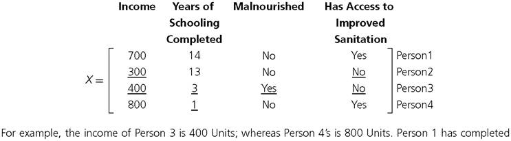
fourteen years of schooling; whereas Person 2 has completed thirteen years of schooling. Person 3 is the only person who is malnourished of all four persons. Two persons in our example have access to improved sanitation. Thus, each row of matrixX contains the achievements of each person in four dimensions, whereas each column of the matrix contains the achievements of four persons in each of the four dimensions. All dimensions are equally weighted and thus the weight vector is w = (0.25,0.25,0.25,0.25). The deprivation cutoff vector is denoted by z = (500, 5, Not malnourished, Has access to improved sanitation), which is used to identify who is deprived in each dimension. The achievement matrix X has three persons who are deprived (see the underlined entries) in one or more dimensions. Person 1 has no deprivation at all.

Based on the deprivation status, we construct the deprivation matrix g⁰, where a deprivation status of 1 is assigned if a person is deprived in a dimension and a deprivation status of 0 is given otherwise.

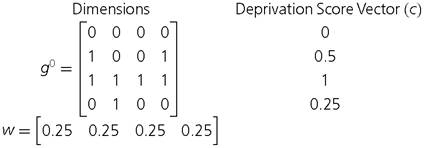
Theweighted sum of dimensional deprivation statuses is the deprivation score (c_i) of each person. For example, the first person has no deprivation and so the deprivation score is 0, whereas the third person is deprived in all

BOX 5.1 (cont.)

dimensions and thus has the highest deprivation score of 1. Similarly, the deprivation score of the second person is 0.5 (= 0.25 + 0.25). The union identification strategy identifies a person as poor if the person is identified as deprived in any of the four dimensions. In that case, three of the four persons are identified as poor. On the other hand, an intersection identification strategy requires that a person is identified as poor if the person is deprived in all dimensions. In that case, only one of the four persons is identified as poor. An intermediate approach sets a cutoff between union and intersection, say, k = 0.5, which is equivalent to being deprived in two of four equally weighted dimensions. This strategy identifies a person as poor if the person is deprived in half or more of weighted dimensions, which in this case means that two of the four persons are identified as poor.

The dual-cutoff identification function has a number of characteristics that deserve mention. First, it is ‘poverty focused' in that an increase in an achievement level x_ij of a non-poor person leaves its value unchanged. Second, it is ‘deprivation focused' in that an increase in any non-deprived achievement x_ij ≥ Zj leaves the value of the identification function unchanged; in other words, a person's poverty status is not affected by changes in the levels of non-deprived achievements. This latter property separates ρ_k from the ‘aggregate achievement' approach which allows a higher level of achievement to compensate for lower levels of achievement in other dimensions. Finally, the dual-cutoff identification method can be meaningfully used with ordinal data, since a person's poverty status is unchanged when an admissible transformation is applied to an achievement level and its associated cutoff.

5.2.4 DUAL-CUTOFF APPROACH AND CENSORING

The transition between the identification step and the aggregation step is most easily understood by examining a progression of matrices. Identification entails two kinds of censoring, each of which follows the application of the two kinds of cutoffs: deprivation and poverty. By applying the deprivation cutoffs to the achievement matrix X, we constructed the deprivation matrixg⁰ replacing each entry in X that is below its respective deprivation cutoff z_j with 1 and each entry that is not below its deprivation cutoff with 0. This is the first censoring, because any level of achievement beyond its deprivation cutoff is effectively being ignored. The deprivation matrix provides a snapshot of who is deprived in which dimension.

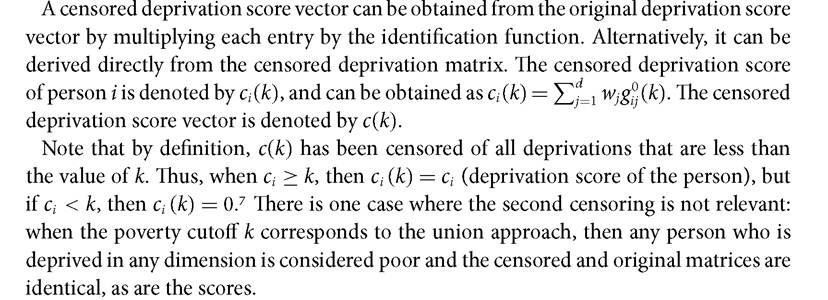
Next, the poor are identified by applying the poverty cutoff k and thus a new matrix can be obtained from the deprivation matrix: the censored deprivation matrix, which is denoted by g⁰(k). Each element in g⁰(k) is obtained by multiplying the corresponding element in g⁰ by the identification function (x_i.; z). Formally, g_i0 (k) = g0 ? ρ_k(x_i.;z) for all i and for all j. What does this mean? If person i is poor and thus ρ_k (x_i.;z) = 1, then the person's deprivation status in every dimension remains unchanged and so does the row containing the deprivation information of the person. If person i is not poor and thus ρ_k (x_i.;z) = 0, then their deprivation status in every dimension becomes 0, which is equivalent to censoring the deprivations of persons who are not poor. This second censoring step is key to the AF methodology. As we will see in subsequent sections, the censored deprivation matrices embody the identification step and are the basic constructs used in the aggregation step.

Although the censored matrices are used to construct multidimensional poverty measures, the original deprivation matrix still provides useful information, as we shall see later in constructing ‘raw' or uncensored deprivation headcount ratios by dimension and analysing their changes over time.

Before moving on to the aggregation step to create the Adjusted Headcount Ratio, let us provide an example of how to obtain the censored deprivation score vector from an achievement matrix in Box 5.2.

BOX 5.2 OBTAINING THE CENSORED DEPRIVATION SCORE VECTOR FROM AN ACHIEVEMENT MATRIX

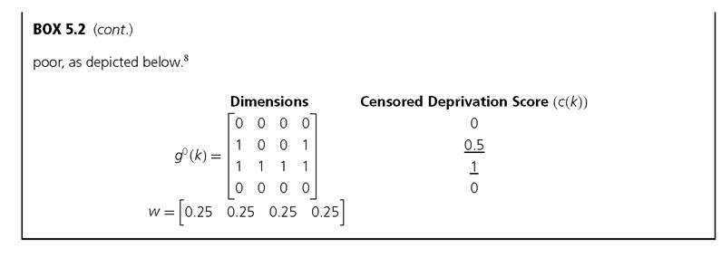
Consider the 4 ? 4 achievement matrix X and the deprivation cutoff vector z in Box 5.1. As earlier, each of the four dimensions receives a weight equal to 0.25 and weights sum to 1. Assume in this case that a person is identified as poor if deprived in half or more of the four equally weighted dimensions, i.e. k = 0.5.

The achievement matrix X has three persons who are deprived in one or more dimensions. Based on the deprivation status, a deprivation matrix g⁰ is constructed in which a deprivation status of 1 is assigned if a person is deprived in a dimension and a status of 0 is given otherwise. The weighted sum of these status values yields the deprivation score of each person c_i.

Note that two persons (second and third) have deprivation scores that are greater than or equal to 0.5. They are considered to be poor (c_i ≥ k), and hence their entries in the censored deprivation matrix are the same as in the deprivation matrix. However, the fourth person has a single deprivation and hence is not poor. This single deprivation is censored in the censored deprivation matrix, which only displays the deprivations of the

⁷In the case of deprivation scores, the poverty cutoff fixes a minimum level of deprivations that identify poverty. This is in contrast to the unidimensional context, where a person is identified as poor if her achievement is below the poverty line.

5.3