LMIs AND WAGE INEQUALITY: AN EMPIRICAL ASSESSMENT
In this section we present an accounting framework and an empirical model aiming to assess the contribution ofLMIs to shaping earnings inequality. Here we face the problem ofiden- tifying who are benefiting from (or disadvantaged by) the action of a specific LMI.
Beforewe have mentioned the stepwise changes introduced by many institutional reforms, which seem to create two-tier systems (Boeri, 2011), implying that the effect of institutions on earnings inequality may significantly differ across age cohorts. To deal with this, the ideal data set would be longitudinal, in order to be able to compute inequality measures over the lifetime of earnings, conditional of attrition in the sample creation. In addition, measuring institutions is not an easy task. Even if we restrict ourselves to the notion of institutions as rules inducing deviations from competitive market equilibria in economic transactions, these rules are still difficult to measure, because they often treat individuals differently or affect their behavior differently (think, for example, of taxes and benefits, which are almost always conditional to family composition—Boeri and Van Ours, 2008). Rules and norms change rather smoothly over time; in the definition used by Boeri (2011), reforms are rarely radical, and therefore it can take a significant amount of time before a minimum detectable effect may be observable. Despite these limitations, a significant literature has studied the correlation between institutional measures and earnings inequality measures (Alderson and Nielsen, 2002; Rueda and Pontusson, 2000; Wallerstein, 1999—more recently Kierzenkowski and Koske, 2012; Scheve and Stasavage, 2009). It exploits, in turn, cross-country and/or over-time variations of the institutions to arrive at estimates of the correlation with earnings inequality. In many instances, the dependent variable (the inequality measures) are derived from secondary sources, and do not always allow for measures that are fully comparable across countries (Atkinson and Brandolini, 2001). Some studies have computed their own inequality measures, relying on existing projects of data harmonization across countries (Atkinson, 2007a,b; Checchi and Garcia Peiialosa, 2008). We have followed here the same line of research, by computing appropriate indices of earnings inequality from SILC and PSID datasets, describedin Section 18.3. Giventhe absence ofnatural experiments to obtain estimates ofthe causal impact ofspecific norms onto the relevant inequality measures, we will obtain at best correlations between institutional measures and inequalities. In Section 18.5.1, we consider a simple accounting scheme in order to discuss the correlation of market equilibria, institutions, and between-group inequality, whereas in Section 18.5.2 we provide a decomposition of the within-group earnings inequality and correlate these measures with proxies for institutions. In Section 18.5.3 we correlate inequality measured across age cohorts with past institutional measures, finding evidence of inequality-reducing impact of unions and minimum wages. Section 18.5.4 discusses the results.A simple accounting scheme is plotted in Figure 18.24, which adopts the core of a scheme presented in OECD (2011) and elaborates on that. It describes the process of generating earnings inequality in an institutional framework. Starting components, individual wages, and hours worked are clearly affected by either the bargaining activity of unions (where/when present and active) and/or by existing regulations (minimum wage, regulation on worked hours). This determines individual labor earnings among the employees, but the total level of employment (and its split between dependent and self-employment) are conditioned by existing taxation as well as by employment protection (because so-called self-employment may disguise dependent employment conditions, especially in the case of a single purchaser). In addition, the generosity of public benefits to those laid-off or unemployed also contributes to reducing earnings inequality in the bottom part of the distribution.
Although we will not proceed further with our analysis in that direction, one should keep in mind that the list of potential institutions affecting earnings inequality at large should consider the household dimension. Half of the sample of the workforce population is concentrated in households where two members are employed (either as dependent or self-employed). As long as their earnings are not perfectly correlated, cohabitation (and expected income sharing) works as a shock absorber. However, one-fourth of the population does not possess this insurance, as they are single-person households who by definition lack such shielding from the unemployment risk.18.5.1 A Simple Scheme to Account for Between-Group Inequality
To frame our theoretical expectations before moving to the econometrics, let us consider a simple model that considers a partition of the population into groups. As such, it may be
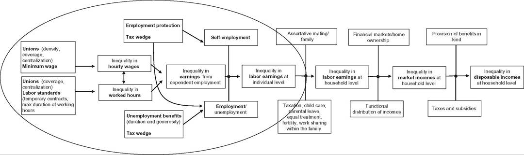
Figure 18.24 Accounting for the basic components of income inequality and the role of institutional measures. Source: Adapted from OECD (2011, box 1).
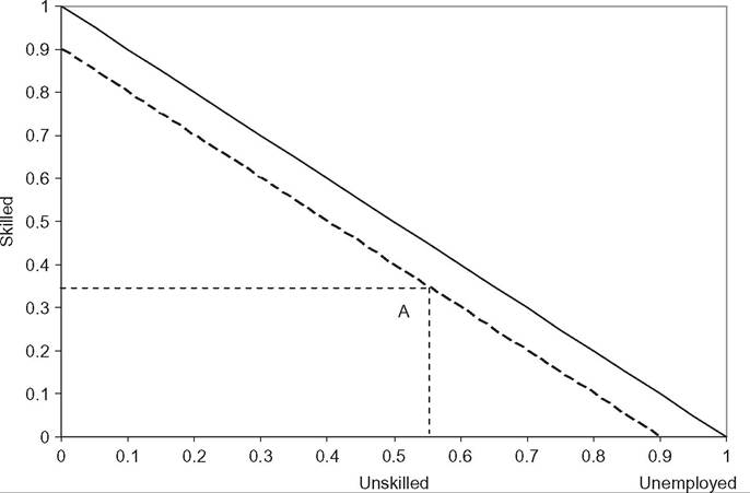
Figure 18.25 The distribution of the population.
considered appropriate to sketch the between-group component of inequality, whereas the between-component incorporates idiosyncratic components (including different marriage attitudes in each group), which are not necessarily connected to the institutional framework. This model builds on Atkinson and Bourguignon (2000) and Checchi and Garcia-Pehalosa (2008). Ifthe workforce is composed by skilled and unskilled workers, a fraction of which may be unemployed, an inequality measure (Gini index) can be expressed (see Box 18.1)

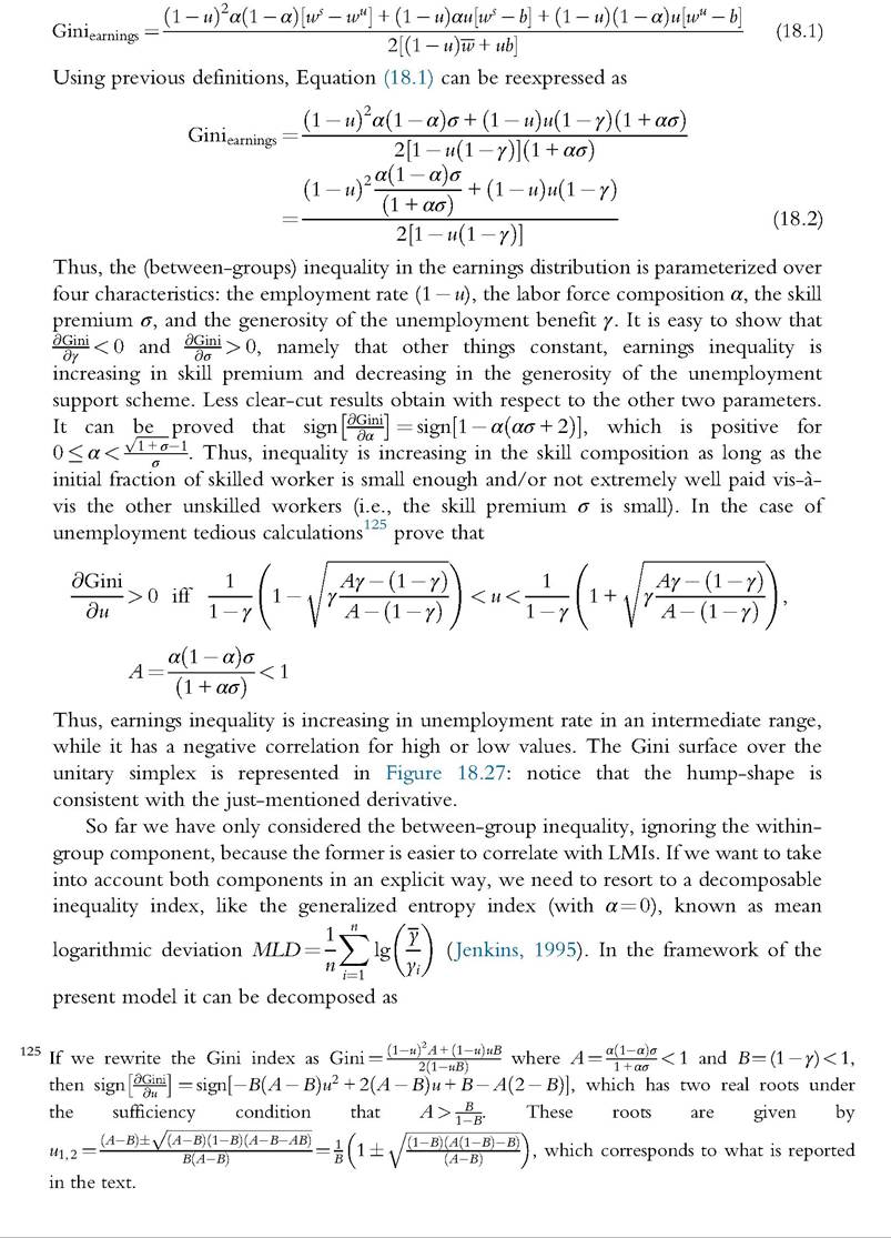
where α indicates the share of skilled workers, σ wage differential between skilled and unskilled wage, u the unemployment rate, and γ the generosity of the unemployment benefit.
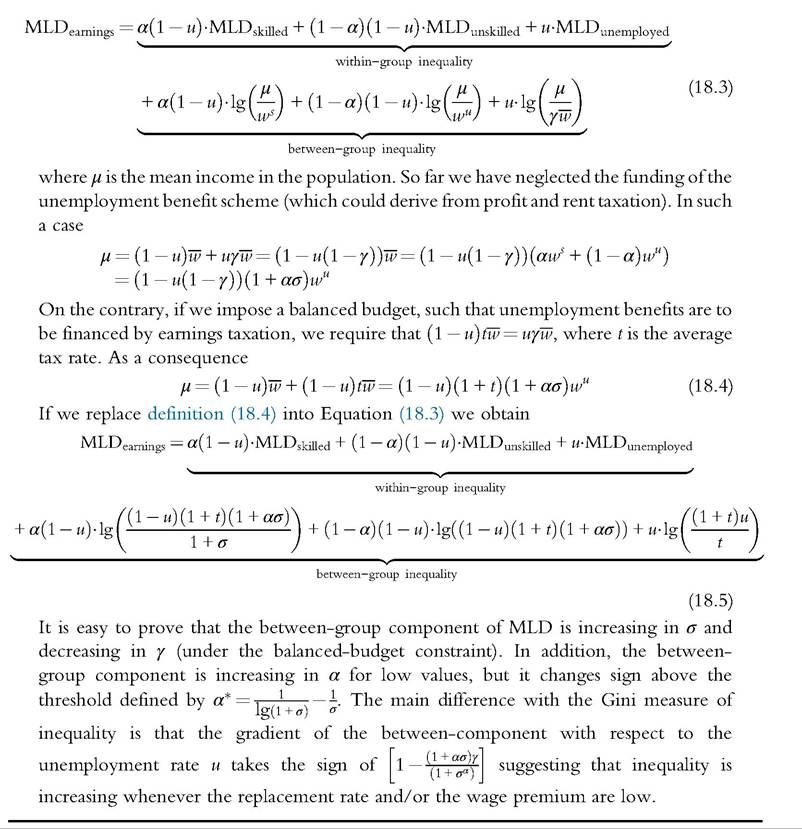
This ideal population can be represented on the unitary simplex (see Figure 18.25), which has its empirical counterpart in our data set (see Figure 18.26). Although it is intuitive that earnings inequality is increasing in skill premium and decreasing in the generosity of the unemployment support scheme (conditional on the replacement rate being less than 100%), the effects of the other two parameters are ambiguous. Inequality is increasing in the skill composition as long as the initial fraction of skilled worker is small enough and/or not extremely well paid vis-a-vis the other unskilled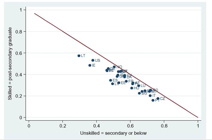
Figure 18.26 The distribution of the employee workforce (aged 20-55)—SILC 2010 and PSID 2011.
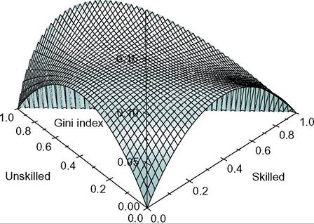
Figure 18.27 Plot of the Gini surface (g ¼0.5, s¼ 2).
workers (i.e., the skill premium is small).[219] Eventually earnings inequality is increasing in unemployment rate in an intermediate range, while it exhibits negative correlation for high or low values (Figure 18.27).
We are now in the position to discuss the relationship between earnings (between- groups) earnings inequality, market determinants, and LMIs. Amongthe Iourparameters identified by the model, one is partly independent from LMI. The skill composition of the employed (parameter α) depends on the interplay between demand and supply of skills. Demand for skill may be related to the technological development of an economy, which, in turns, relates to the international distribution of production and the possibility of off-shoring (Acemoglu and Autor, 2011,2012). The supply of skills is the output of the educational system of a country, combined with expectations regarding wage premia. If we extend the notion of institutions to include educational systems, then this is the first determinant of wage inequality, which is nonlinearly related to earnings inequality (Leuven et al., 2004).
Given intergenerational persistence in educational choice, the skill composition of the labor force changes rather smoothly across generations, and can be taken as given, at least in the short run.By contrast, the return to skill (parameter σ) is jointly affected by competitive market forces and by institutions. In a competitive environment, this relative wage should be negatively correlated with the relative supply, as is slightly the case in Figure 18.28 (Katz and Autor, 1999). However there are significant deviations from such a relationship, which, among other factors, depend on the bargaining activity of unions (typically pursuing an egalitarian stance, aiming to tie wages to jobs and not to people—Visser and
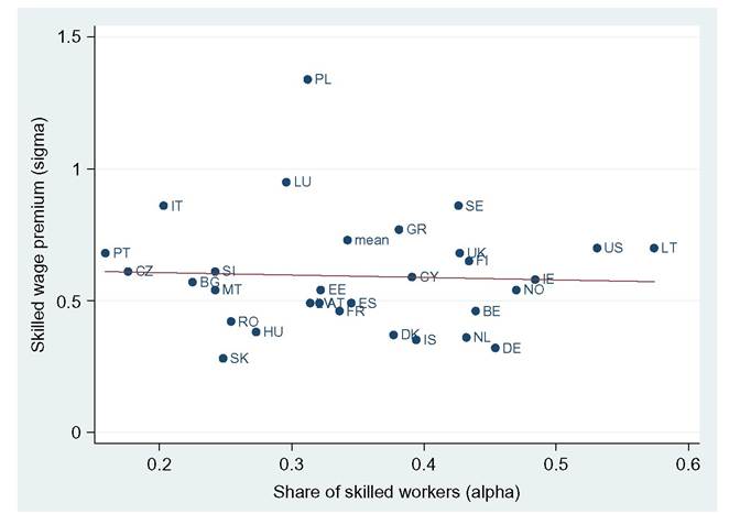
Figure 18.28 Return to skills and skill availability for dependent employees (aged 20-55)—SILC 2010 and PSID 2011.
Checchi, 2009; see also the role of wage scales described by Oliver, 2008) as well as the presence and coverage of minimum-wage legislation.
The unemployment benefit (parameter γ) has an Uncontroversial effect of reducing earnings inequality when unemployed people are counted in. However, there is a general consensus that it has also a detrimental effect on the incentive to work, thereby raising the unemployment rate. Because the unemployment benefit can be thought of as a proxy for the outside option in wage bargaining or efficiency wage models, it also creates an upward wage push, which contributes to a positive correlation between benefit and unemployment. The overall effect is therefore = ¾Gιnι I + which
γ γ u=constant γ
can be either positive (for a high level of unemployment and/or a weak elasticity of unemployment to benefit) or negative (for a low level of unemployment and/or a high elasticity of unemployment to benefit). In our sample, the correlation tends to be positive (see Figure 18.29—however, this concerns short-run unemployment rates, whereas such a correlation should be studied using multiperiod unemployment rate in order to dispense with cyclical fluctuations).
Once again, this is not the unique determinant of the unemployment rate (parameter u), because in a more general equilibrium model it depends on the state of the aggregate demand as well as on the average labor cost, which should incorporate the tax wedge. In addition, it may also be correlated with many other LMI variables, sometimes referred as determinants of the nairu (Nickell, 1997).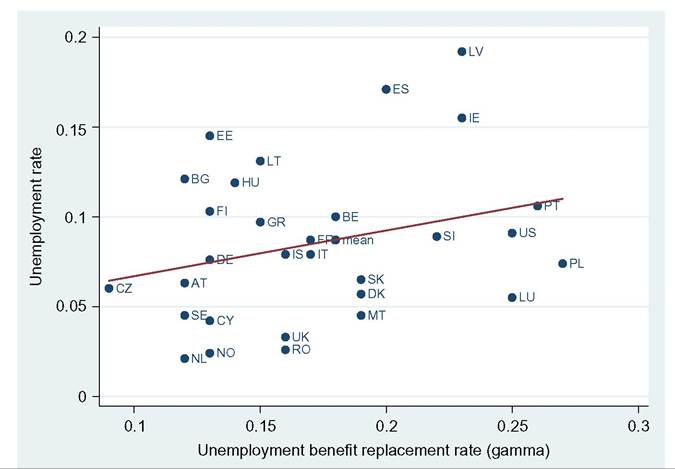
Figure 18.29 Unemployment benefit and unemployment rate—SILC 2010 and PSID 2011.
Still on the side of between-group inequality, we have purposely ignored the functional distribution of income between profit and wages, even though some of these parameters may be correlated to the labor share in the value added. Checchi and Pehalosa (2008) have shown that the same LMI affecting the functional distribution of value added, also affect the distribution of income sources at the individual level, thus modifying income inequality at the aggregate level.
Ifwe are to check the predictive ability of this simple model, we can use observed sample parameters (a, σ, u, γ) to predict earnings inequality in each country, well aware that this captures only the between-group component. We define as skilled workers all employees holding a postsecondary degree, and compute the skilled wage as their mean wage. Correspondingly, we define as unskilled all the remaining employees (and obtain their wage); finally, we compute the unemployment share and their mean benefit. The relevant parameters, which are needed for the between-group inequality measures, are reported in Table 18.A4. In column 10, we report the estimated Gini, which has to be compared
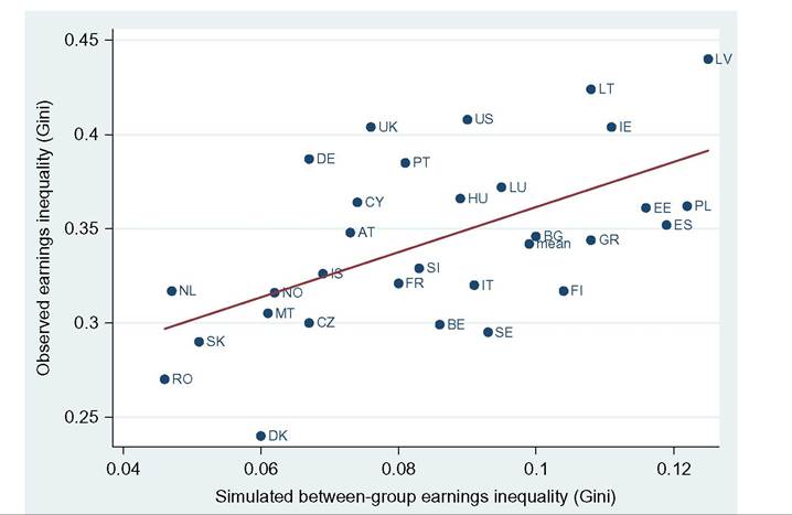
Figure 18.30 The between-group component of earnings inequality—SILC 2010 and PSID 2011.
with the actual one computed on the same data set in column 11. The two coefficients are highly correlated (rank correlation coefficient is 0.57).
Using the Gini index computed over four parameters, we can claim that the between- group component accounts for almost one-third of overall earnings inequality, the remainder being attributable to individual heterogeneity (age, gender, finer partition of educational attainments—including variations of hours). It is rather surprising that such a simple model, based on four parameters only, is able to account for a significant portion of the observed cross-country differences in earnings inequality. Looking at Figure 18.30 we notice that some countries (lying to the right of the regression line) are characterized by higher-than-the-mean between-group inequality (or lower-than-the-mean overall earnings inequality): not surprisingly the Nordic and the Mediterranean countries (except Portugal) are on this side, indicating that in these countries institutions may help to reduce the corresponding within-group inequality. On the left side of the regression line, however, we find the liberal market economies (United States, United Kingdom, and Ireland) and some transition economies (Latvia, Lithuania, and Hungary) as well as some 
continental European country (such as Germany and the Netherlands). These countries are characterized by individual rather than collective wage setting, thus raising the between-group component of earnings inequality.
18.5.2 The Within-Group Inequality and the Role of LMIs
We now consider the within-group component of inequality. To obtain an exact decomposition of earnings inequality for employees, we abstract from self-employment (we think it is potentially affected by existing labor market regulations, but it often also records negative incomes that are not easily dealt by inequality measures), and we restrict ourselves to individuals aged below 55 (to minimize country differences attributable to a different extent of early retirement127) who receive either a positive income from dependent employment or from unemployment benefit. Using the mean log deviation to decompose earnings inequality, we find that on average the between-component accounts for one-fifth of the observed inequality, being highest in Portugal (30%), Hungary (28%), and Slovenia (28%) and lowest in Sweden (7%), Norway (8%), and the Netherlands (11%) (see Table 18.3).
The within-group component follows common patterns: inequality is highest among the unemployed,128 but its contribution to the within-group component is limited, the country average being 16%. Skilled workers are characterized by higher earnings inequality than the unskilled ones, and this is not surprising once we consider that their wage will more frequently be determined by individual bargaining. The unskilled workers (who on average comprise 57% of the workforce) do contribute half of total within-group inequality, and it is here that we may expect to find the strongest impact of LMIs (especially the minimum wage and bargaining activity of unions).129
Table 18.3 Earnings inequality decomposition—dependent employees or unemployed (mean log deviation)—SILC 2010 and PSID 2011
Decomposition of total inequality Decomposition of the within-group component
| Overall yearly gross earnings inequality | Between group inequality | Within group inequality | Population share of skilled workers | Inequality in yearly gross earnings of skilled workers | Population share of unskilled workers | Inequality in yearly gross earnings of unskilled workers | Population share of unemployed workers (receiving a positive benefit) | Inequality in unemployment benefits (conditional on being unemployed) | |
| Austria | 0.234 | 0.031 | 0.203 | 0.321 | 0.223 | 0.616 | 0.181 | 0.063 | 0.327 |
| Belgium | 0.179 | 0.048 | 0.131 | 0.439 | 0.124 | 0.461 | 0.119 | 0.100 | 0.214 |
| Bulgaria | 0.241 | 0.046 | 0.195 | 0.225 | 0.176 | 0.654 | 0.161 | 0.121 | 0.410 |
| Cyprus | 0.263 | 0.031 | 0.232 | 0.391 | 0.255 | 0.567 | 0.214 | 0.042 | 0.270 |
| Czech | 0.184 | 0.033 | 0.151 | 0.176 | 0.171 | 0.764 | 0.119 | 0.060 | 0.494 |
| Republic Denmark | 0.129 | 0.016 | 0.113 | 0.376 | 0.111 | 0.566 | 0.101 | 0.057 | 0.243 |
| Estonia | 0.270 | 0.033 | 0.237 | 0.322 | 0.200 | 0.532 | 0.194 | 0.145 | 0.475 |
| Finland | 0.204 | 0.049 | 0.155 | 0.434 | 0.145 | 0.462 | 0.132 | 0.103 | 0.294 |
| France | 0.229 | 0.031 | 0.198 | 0.336 | 0.197 | 0.576 | 0.173 | 0.087 | 0.367 |
| Germany | 0.334 | 0.069 | 0.265 | 0.454 | 0.234 | 0.470 | 0.276 | 0.076 | 0.381 |
| Greece | 0.224 | 0.031 | 0.193 | 0.381 | 0.197 | 0.522 | 0.164 | 0.097 | 0.328 |
| Hungary | 0.250 | 0.071 | 0.179 | 0.273 | 0.206 | 0.608 | 0.150 | 0.119 | 0.262 |
| Iceland | 0.218 | 0.027 | 0.191 | 0.394 | 0.169 | 0.527 | 0.178 | 0.079 | 0.384 |
| Ireland | 0.316 | 0.048 | 0.268 | 0.484 | 0.250 | 0.361 | 0.233 | 0.155 | 0.406 |
| Italy | 0.224 | 0.027 | 0.197 | 0.203 | 0.205 | 0.718 | 0.169 | 0.079 | 0.436 |
| Latvia | 0.418 | 0.076 | 0.342 | 0.314 | 0.279 | 0.495 | 0.261 | 0.192 | 0.653 |
| Lithuania | 0.377 | 0.061 | 0.316 | 0.574 | 0.295 | 0.296 | 0.248 | 0.131 | 0.566 |
| Luxembourg | 0.260 | 0.060 | 0.200 | bgcolor=white>0.2960.205 | 0.649 | 0.196 | 0.055 | 0.213 | |
| Malta | 0.199 | 0.029 | 0.170 | 0.242 | 0.179 | 0.713 | 0.150 | 0.045 | 0.453 |
| Netherlands | 0.200 | 0.023 | 0.177 | 0.432 | 0.172 | 0.547 | 0.167 | 0.021 | 0.563 |
| Norway | 0.230 | 0.018 | 0.212 | 0.470 | 0.204 | 0.505 | 0.200 | 0.024 | 0.605 |
Continued
Table 18.3 Earnings inequality decomposition—dependent employees or unemployed (mean log deviation)—SILC 2010 and PSID 2011—cont'd
Decomposition of total inequality Decomposition of the within-group component
| Overall yearly gross earnings inequality | Between group inequality | Within group inequality | Population share of skilled workers | Inequality in yearly gross earnings of skilled workers | Population share of unskilled workers | Inequality in yearly gross earnings of unskilled workers | Population share of unemployed workers (receiving a positive benefit) | Inequality in unemployment benefits (conditional on being unemployed) | |
| Poland | 0.253 | 0.038 | 0.215 | 0.312 | 0.226 | 0.614 | 0.188 | 0.074 | 0.387 |
| Portugal | 0.259 | 0.078 | 0.181 | 0.159 | 0.246 | 0.734 | 0.163 | 0.106 | 0.204 |
| Romania | 0.121 | 0.032 | 0.089 | 0.254 | 0.111 | 0.720 | 0.078 | 0.026 | 0.176 |
| Slovak | 0.180 | 0.029 | 0.151 | 0.248 | 0.172 | 0.687 | 0.113 | 0.065 | 0.476 |
| Republic | |||||||||
| Slovenia | 0.229 | 0.064 | 0.165 | 0.242 | 0.189 | 0.669 | 0.116 | 0.089 | 0.471 |
| Spain | 0.249 | 0.057 | 0.192 | 0.345 | 0.177 | 0.483 | 0.171 | 0.171 | 0.284 |
| Sweden | 0.230 | 0.016 | 0.214 | 0.426 | 0.245 | 0.530 | 0.166 | 0.045 | 0.484 |
| United | 0.306 | 0.058 | 0.248 | 0.427 | 0.261 | 0.541 | 0.231 | 0.033 | 0.359 |
| Kingdom | |||||||||
| United | 0.339 | 0.045 | 0.294 | 0.483 | 0.310 | 0.468 | 0.271 | 0.049 | 0.347 |
| States | |||||||||
| Average | 0.245 | 0.044 | 0.201 | 0.340 | 0.203 | 0.575 | 0.174 | 0.085 | 0.388 |
Ifwe now consider the potential role of LMI in shaping the wage distribution within workers’ types, we do expect a differential impact according to the way in which different workers are affected.[220] We spent some effort to collecting consistent information on institutional variables for the same countries, mostly from various OECD data sets. We tried to build long series in order to match individuals of different age cohorts to the institutional setup prevailing either at the beginning of their work careers or during their entire career. Data sources and descriptive statistics are in Appendix C.
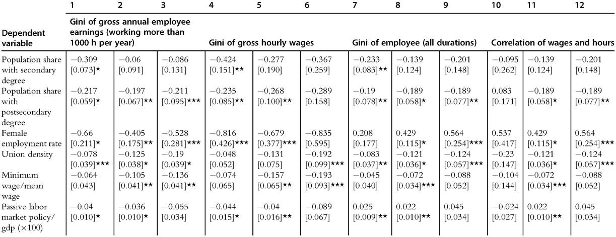
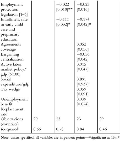
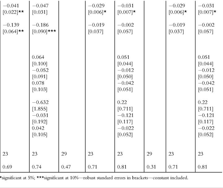
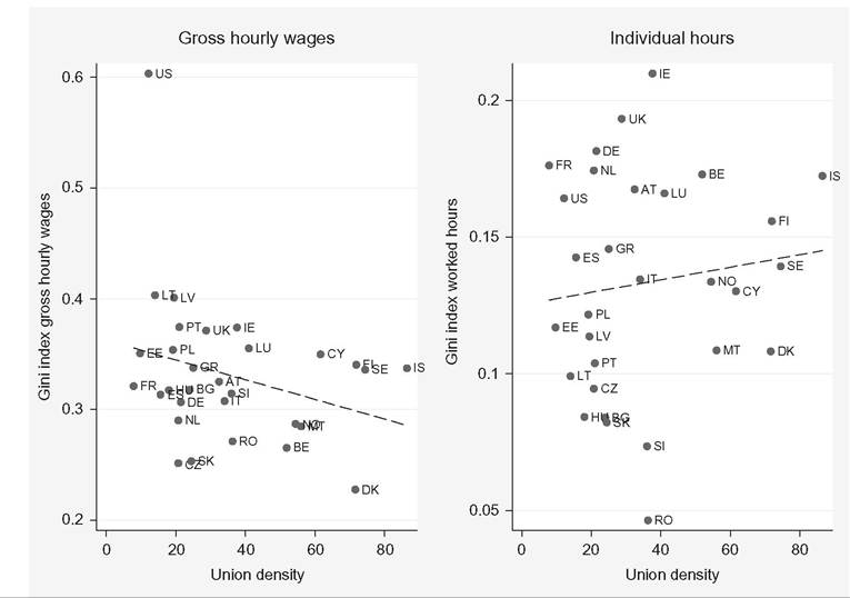
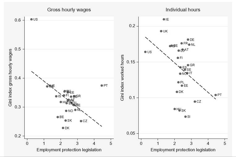
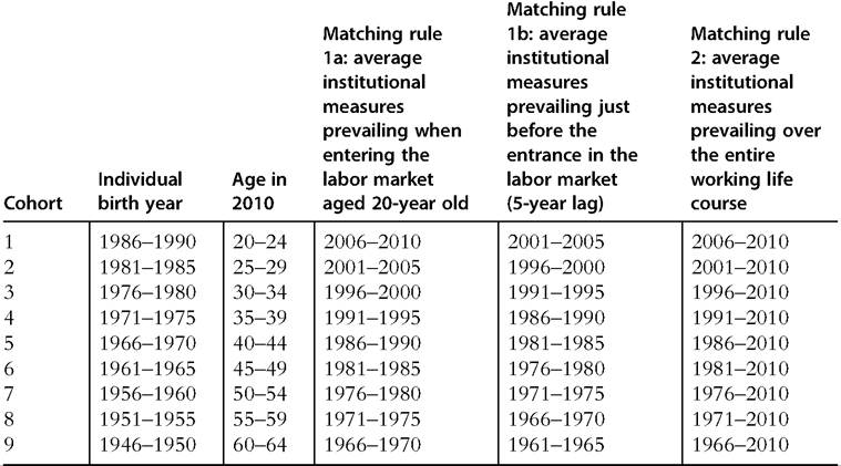
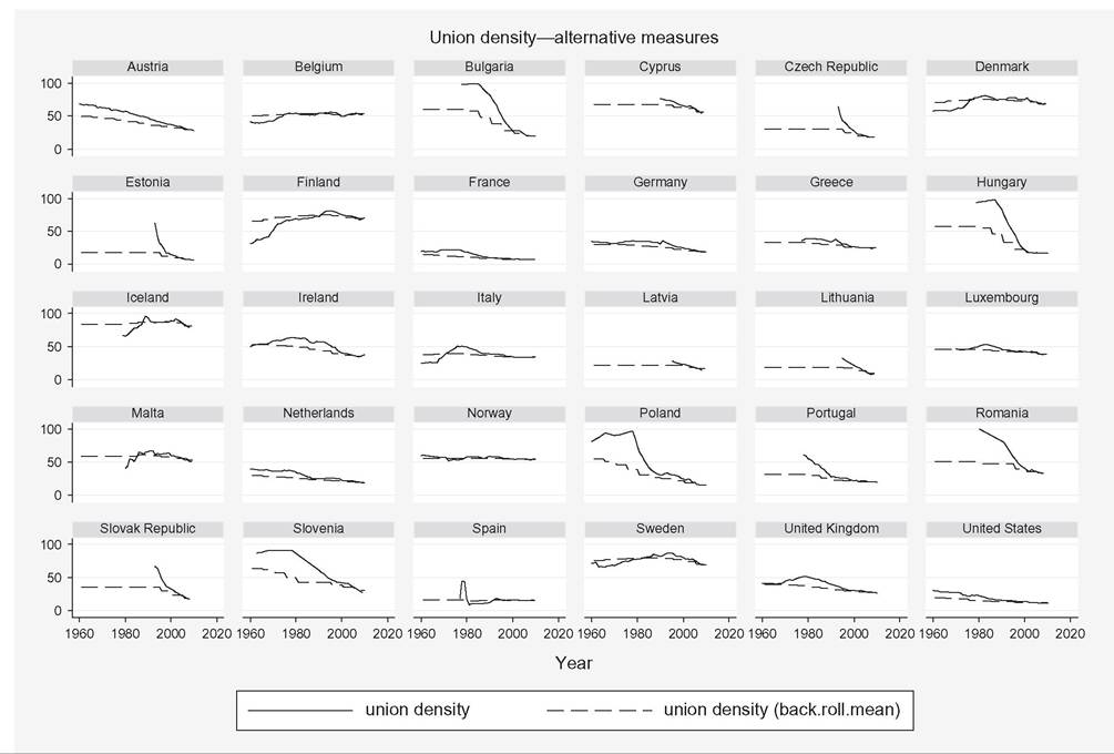
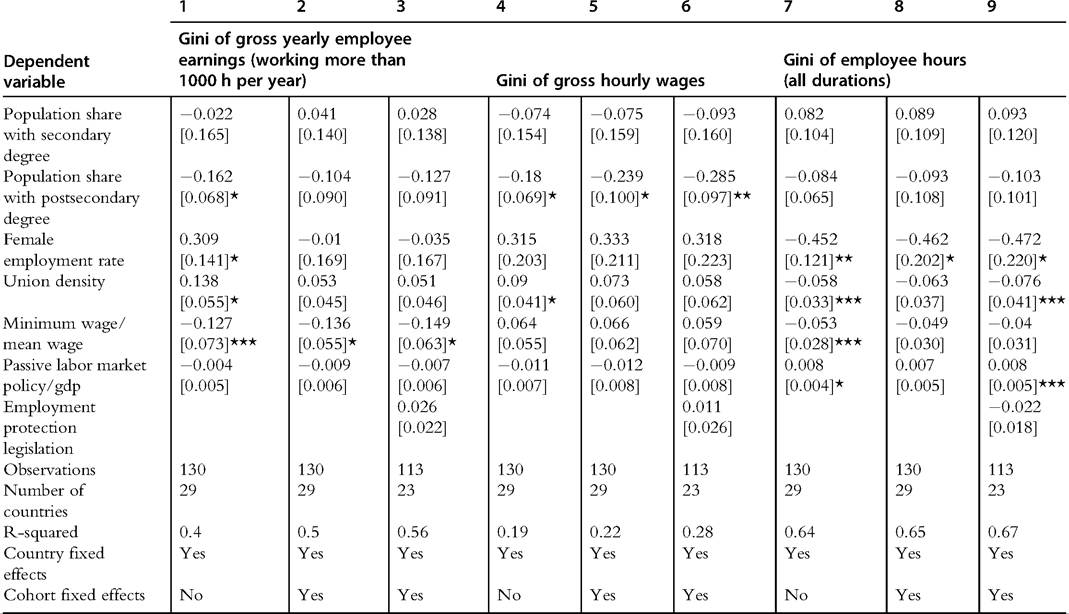
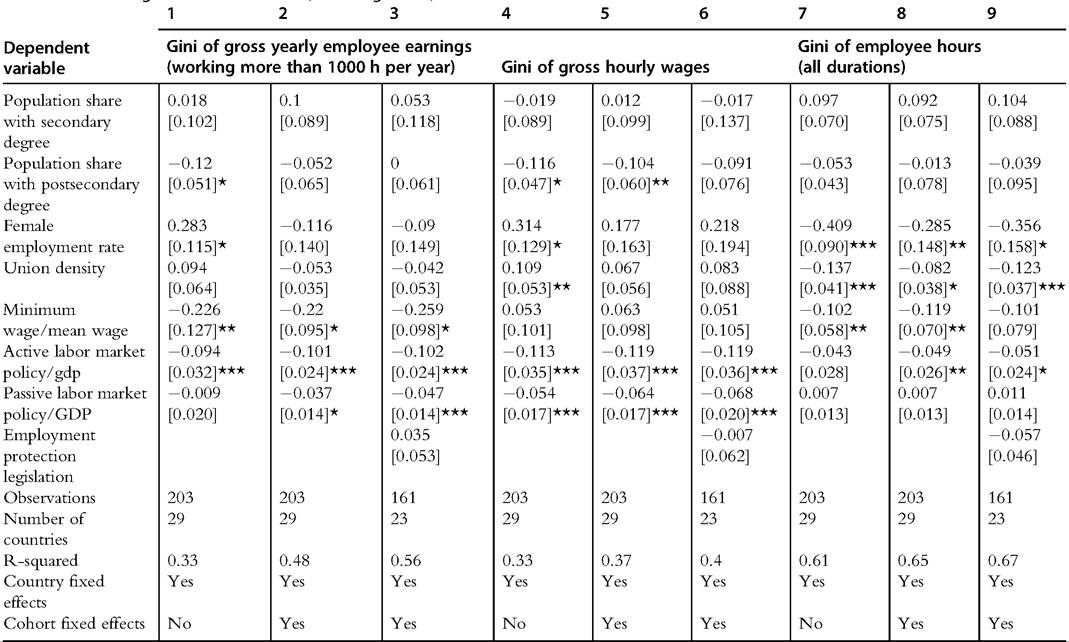
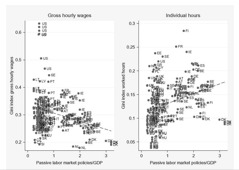
Table 18.4 summarizes our theoretical expectations, mostly deduced from the existing literature. Betcherman (2012) reviews the empirical literature on the correlation between different institutional dimensions and earnings inequality. He concludes that the minimum wage is the less contentious among the institutional impact, being associated to an improvement in the bottom tail of the wage distribution, at least for the formal sector. Neumark and Wascher (2008) do not contest the inequality-reducing impact of minimum wage (by creating a spike at the relevant threshold and/or inducing upward spillover effect across the entire wage distribution), though they stress the contemporaneous disemployment effect on low-wage earners, raising doubts about the overall effect on inequality at household level.[221] [222] [223] The effect of unions is mixed, combining a reduction of within-group inequality (among formal dependent employment, especially in terms of skill premium— Koeniger et al., 2007) and a potential increase in the wage gap between union-covered sectors and nonunion-covered sectors (including informal employment). Using crosscountry data, Visser and Checchi (2009) find that union presence is associated with lower within-group inequality, because both the gender gap and the return to education are negatively correlated with union density.132,133 As a consequence, the skill premium declines, both as a result of wage compression and as a consequence of the incentives to over-invest in education. In addition, union presence is also associated to Overall impact on earnings • Reduces gender wage gap, thus favoring work-sharing within the family and female participation • Increases long-term unemployment • Discourages labor market entry of marginal workers (young, women) • Raises the outside option, thus augmenting the bargaining power of unions • Lowers the incentive to job search • Even within the household, EITC (earned income tax credit) measures may favor joint participation of spouses to the labor market, especially when part time is easily available • Increasing female participation, it brings in additional workers into employment • Ambiguous (due to a compositional effect) unemployment, though correlation may go in different directions: union density seems associated with higher unemployment (Bertola et al., 2007; Flaig and Rottmann, 2011; Nickell et al., 2005), and centralized bargaining seems to attenuate this negative effect (Bassanini and Duval, 2006; Nickell, 1997—see also Glyn et al. (2003) for a critical review ofthese results). Thus, the overall effect ofunions on earnings inequality remains uncertain. The results of employment protection legislation are less clear-cut. OECD (2011, 2012) show that EPL and wage coordination have a negative effect on earning inequality, while tax wage and wage coverage have a positive effect. The proposed rationalization is that unskilled workers are favored by firing restriction, raising their relative bargaining power relative to skilled ones.[224] [225] Unemployment benefits, active labor market policies, and the tax wedge may play an indirect role, via the impact on aggregate employment (or unemployment). The tax wedge in particular has been found to be significantly and positively correlated to the unemployment rate (Flaig and Rottmann, 2011; Nickell et al., 2005). But these two institutions also affect different groups of workers in different ways, especially along the gender divide (Bertola et al., 2007): as a consequence, they may impact on the household distribution of earnings via changes in the redistribution of work opportunities within the family. In addition, when aiming to decompose the contribution to inequality associated with hourly wages and hours worked, the legal framework (limitation to part-time, family, or individual taxation) may lead to opposite impacts on labor supply, the corresponding employment and wage outcomes. Possibly for these reasons, we have not found consensus on this dimension in the literature, and therefore we will let the data speak. Work redistribution within the household may also be affected by parental leave opportunities and child care provisions (Thevenon and Solaz, 2013). As long as these institutional dimensions favor female participation, they should reduce earnings inequality measured at the household level, but they may increase inequality at the individual level, owing to a larger fraction of part-timers in the economy. However, these results are conditional on parental leave not exceeding a specific threshold, because otherwise it may produce a reduction in labor supply.[226] In addition, as long-mandated parental leave may raise female supply in the labor market, it may also exert a downward pressure on their relative wage, thus contributing to increased inequality (which, however, is not found in the limited data analyzed by Thevenon and Solaz, 2013). Also in such a case, we may let the data speak. A serious problem in assessing the impact of single institutions on labor market outcomes is that some institutions are likely to interact with each other, in a positive or in a negative way. Consider, for example, the role of workers’ unions, which is typically correlated in a negative way to earnings inequality. The presence of unions is strengthened by employment protection legislation, but is weakened by the presence of minimumwage provisions.[227] Similarly, the tax wedge may have a significant impact on employment in a country where the (after-tax) minimum wage is relatively high because part of the wedge will be passed on to wages at a higher level. In some countries (such as France and Belgium) rebates on payroll taxes for low-wage workers significantly impact on their employability. Addressing the issue of institutional complementarity opens up another set of literature, which is typically analyzed by political economy (Amable, 2003; Hall and Soskice, 2001). From an empirical point of view it does require a sufficient number of degrees of freedom (either in terms of variety of countries or in terms of repeated observations over the same country). Just as descriptive evidence, the sample bivariate correlations between the inequality measures presented in Table 18.4 and the LMIs described in Appendix C are presented in Table 18.5.[228] Exploiting the decomposability of the Mean Log Deviation, we have considered six dimensions of earnings inequality: its overall measure, the decomposition into between-group and within-group, and the contributions to the within-component attributable to each group of workers (skilled, unskilled, and unemployed).[229] They confirm that union presence (either measured by union density or by coverage) may contribute to reducing earnings inequality, though in a different way. Union density seems statistically correlated with the between-group component, whereas the coverage of collective agreements (which assures equivalent treatment of all workers) exhibits a negative correlation with the within-component. Similar negative correlations are exhibited by employment protection with respect to the skilled worker group; analogously, parental leave facilities are negatively correlated to skilled wage inequality. It is Table 18.5 Correlation between labor market institutions (averages 2001-2010) and different component of earnings inequality (MLD)—SILC 2010 and PSID 2011 benefit 30 countries—*significant at 10%. interesting to note that the generosity of the unemployment benefit seems to contribute positively to the inequality component attributable to the unemployed (even if we are unable to distinguish whether this is due to an increase of the unemployment rate or to a different distribution within the group). Not surprisingly, household or individual taxation does not affect wage inequality, because it may be ineffective in modifying household labor supply (Dingeldey, 2001). Active and passive labor market policies seem mostly effective in reducing the within-component of the earnings inequality of unskilled workers. Overall these results are not satisfying in terms of statistical significance, suggesting that isolating a single institution at a specific point in time (even though here we are considering a decennial average) may not be the best strategy to investigate the association between inequality and institutions. Though it may sometimes be inevitable for empirical reasons, it does seem advisable to consider the degree of embeddedness of individual institutions in a collection of institutions to see whether one can lay more weight on analytical results obtained for one institution compared to another. For example, the strong legal nature of an institution may enhance its standalone effect. In addition, bivariate correlations are sensitive to the criticism of spurious correlation and also to omitted-variable bias. For this reason we now consider more robust methods to study the impact of institutions on earnings inequality. 18.5.3 Empirical Assessment 18.5.3.1 Cross-Sectional Approach One crucial issue in the analysis of the role of LMI in shaping earnings inequality is the match of inequality computed from microdata to the corresponding institutional measures. If we correlate current inequality measured over workers of different ages (who therefore have been staying in the labor market for different durations) to the current union density (which is computed over the workers who are currently working) we are simply considering “industrial relations” regimes, without any claim of causality in one direction or the other. Such an exercise is conducted in Table 18.6, in which we consider three different dimensions of inequality (yearly earnings from dependent employment, hourly wages, and worked hours by dependent employees). In accordance with our previous between-group inequality decomposition (see Section 18.5.2), for each dimension we consider two market phenomena that are correlated with market forces: level of qualification of the labor force and level of employment (better captured by the female employment rate). 0 In all cases an increasing level of education in the 140 Actually the skill level of the labor force is the joint outcome of the demand for education of the population and the institutional supply of schooling; however, replacing it with some measure of the strength of the institutional push toward education (such as the years of compulsory education) did not prove statistically significant. Table 18.6 Gross earnings inequality (SILC 2010-PSID 2011) against market and labor market institutions (2001-2010) Effects—OLS Figure 18.31 Earnings inequality (SILC 2010-PSID 2011) and union density (average 2001-2010). labor force is negatively and significantly associated with inequality. Similarly, it occurs for wages, but not for hours: not surprisingly, when more women enter the labor market, the working hours regime as a whole becomes more diversified.[230] [231] 142 When we introduce institutional measures to capture deviations from market equilibrium, we identify a subset of institutions that are significantly correlated with different inequalities (see columns 2-5-8 of Table 18.6). Union density has a negative association with yearly earnings, hourly wages, and hours: this captures different dimensions of union presence (such as coverage or wage centralization, which are not statistically significant ). Although the unconditional correlation with worked hours appears positive (see Figure 18.31), once we control for compositional effects it turns negative (despite a rather small magnitude). A second institutional dimension with a statistical negative correlation with earnings inequality is the presence and the level of minimum wages. However, as discussed in Appendix C, this institution is present only in a subset of countries, while in others this role is played by legislative or judicial extension of the union-bargained wage. In addition, there are often derogations for marginal workers, which are not captured by this measure. Nevertheless, the mere existence of a legal floor to downward flexibility of wages contributes to the containment of inequality. The third institutional dimension deals with unemployment benefit, whose theoretical expectation is ambiguous due to a potential enhancing effect on the unemployment rate. The replacement rate does not exhibit a statistically significant correlation, whereas the overall public expenditure on passive labor market policies is negatively correlated with earnings and wage inequalities, and positively with hours inequality.[232] This suggests that transferring money to members of the labor force (which constitutes our sample of investigation) reduces inequality in terms of revenues, but on the other side allows for the continuation of unequally distributed job opportunities. A fourth dimension is connected to the employment protection.[233] Not surprisingly, its correlation is strongest with the distribution of work: the more regulated the labor contract, the more equal is the distribution of worked hours. Because employment protection and union activities tend to be complements (Bertola, 2004), it is not surprising to find an analogous negative correlation with earnings and wage inequality, as clearly shown in Figure 18.32. Still restricting our examination to the subsample of OECD countries, we find some statistical evidence of a negative correlation of earnings inequality with child care attendance, interpreted as a proxy for child care availability. On a theoretical ground, we do expect a larger female participation in the labor market and an evener distribution of external work opportunities in the couple: both should have an impact on the hours inequality, which, however, do not appear in the data. The negative correlation with earnings inequality could capture some unobservable dimension of welfare provision, which is typically associated to lower inequality (though a direct measure of it, given by social expenditure, does not come out statistically significant).[234] Despite the limited degrees of freedom, these are the only institutional features that correlate with statistical significance with various dimensions of earnings inequality. Against the potential objection of omitted variables, we have also introduced all measures that we have collected (see columns 3-6-9 of Table 18.6), without finding any other statistical correlation. However, despite the richness of the institutional framework, a simple cross-country regression such as the actual one does not provide an incontrovertible evidence of LMIs contributing to shape earnings inequality. To this end, we now move to exploit cohort variation in inequalities. Figure 18.32 Earnings inequality (SILC 2010-PSID 2011) and employment protection (average 2001-2010). In columns 10—11—12 of Table 18.6 we have considered as a dependent variable the correlation computed at the country level between hourly wages and worked hours, following the idea that higher correlation (in absolute terms) may reduce earnings inequality (as long as this correlation does not simply capture spurious correlation—see again Figure 18.22 and the discussion there). We find a negative correlation with both union density and employment protection legislation, suggesting that in a highly regulated labor market (due to firing restrictions and/or active union presence) the working poor obtain partial compensation of their weak command in the labor market by extended (or just complete) working hours. 18.5.3.2 Longitudinal or Pseudo-Longitudinal Approach Aiming to obtain more statistically robust results, we need to exploit cross-country and within-country variations of inequality and institutions, to be able to dispense with unobservables by means of appropriate country and time-fixed effects. If data were available, one could take repeated cross sections for each country, compute inequality Table 18.7 Matching rules between inequality measures and institutional variables measures of the relevant population in each survey, and match them with the prevailing institutional measures. Unfortunately, cross-country comparable surveys for the countries under analysis do not go back more than a couple of decades, and this has led us to pursue an alternative strategy. Because we need to match individuals belonging to different age cohorts, who entered the labor market in different years, to institutional profiles that are relevant for their wage determination, we need to discuss the appropriate matching rule. One possibility would match individuals to the institutions prevailing at the time of their entrance into the labor market (see matching rules 1a and 1b in Table 18.7). This implies that the current difference between a person’s wage and the wages of his or her coworkers may be affected by the bargaining activity exerted by the unions 30 years ago. As long as wages are highly persistent (due to seniority rules and/or automatic adjustment clauses) this may be considered a viable assumption. An alternative possibility considers both institutional persistence (institutions are slow-changing variables) and different exposure to an institutional environment (variable treatment). In this second perspective, older individuals are supposed to have been exposed to an institutional framework that has been (on average) available over their entire working life (see matching rule 2 in Table 18.7). In such a case, the current difference between someone’s wage and the wages of his or her coworkers has been affected by the bargaining activity exerted over the past 30 years. To appreciate differences in the institutional measures according to the different matching rules, Figure 18.33 plots the Figure 18.33 Alternative measures of exposition to institutions: union density. contemporaneous union density (solid line) and the backward (moving) mean according to the third matching rule (dashed line): although the former is more volatile, the latter “keeps” a smoothed memory of past dynamics. Both strategies are approximations because they induce measurement errors in the dependent variables (measuring wage inequality by age cohort is used as proxy for overall inequality measured in the past). However, they have the advantage of covering a long time span, allowing greater variability in the institutional measures. Irrespective of the chosen matching, by treating our cross section as a pseudo-panel we significantly augment the degrees of freedom in the estimation. The different time coverage of institutional measures yields an unbalanced panel, where we control for country and cohort fixed effects. The errors are clustered at the country level. As a consequence, our results are more robust than the previous cross-section estimates reported in Table 18.8. As long as the fixed effects clean away all the other sources of confounding variations, we use cross-country and life-cycle variations in inequality for identifying the contribution of institutions to shape the earnings distribution. The contemporaneous insertion of several institutional measures allows for the identification of each specific contribution, other institutions and sample composition kept constant. We have decided to exclude the two oldest cohorts, inasmuch as information on institutions in the 1960s is available only for union density and unemployment benefit. In addition, retirement rules vary across countries, introducing large variations in the employment rate for these age cohorts.[235] In Table 18.8 we present the estimates corresponding to the matching rule 1a (individual matched to the institutions prevailing when entering the labor market—the other matching rule 1b gives similar results on a shorter sample size, and is not reported for brevity). The structure of Table 18.8 resembles the previous Table 18.6 but leaves out the analysis of the correlation between hours and wages. We consider three measures of inequality (yearly earnings for full-time workers, hourly wages, and hours worked) and for each of them we control for educational attainment in the labor force and female participation. In both cases they exert a negative impact on inequality, despite the weaker statistical significance of education. For each dependent variable we consider three specifications: country fixed effects (columns 1-4-7), country and cohort fixed effects (columns 2-5-8), and country and cohort fixed effects including OECD indicator for employment protection, which excludes non-OECD members (columns 3-6-9).[236] Table 18.8 Gross earnings inequality (SILC 2010-PSID 2011) against market and labor market institutions (1975-2010) effects—OLS—longitudinal cohort data (matching rule 1a) Robust standard errors clustered by countries in brackets—; *significant at 5%; **significant at 1%; ***significant at 10%. In this framework we find only partial support to our previous findings with crosssectional analysis. Focusing on a model that includes both country and cohort fixed effects, there is some evidence of a negative impact of unions on the distribution of work (column 9) and of a stronger impact of the minimum wage on earnings inequality. Contrary to previous results, passive labor market policies do not reach statistical significance for their negative impact on earnings and wage inequality, but register some positive impact on the Gini index for hours worked. Other institutional variables (such as the tax wedge, unemployment benefit, parental leave, and active labor market policies), which are constantly nonsignificant are not reported for brevity. The same results are reinforced when we adopt the second matching rule, as shown in Table 18.9. The different data organization significantly extends the sample, and this allows for a more precise identification of the effects (see, for example, the unconditional correlation with passive labor market policies, depicted in Figure 18.34). Union density is now clearly reducing inequality in hours, and the minimum wage reduces inequality both in earnings and hours. In addition to the negative contribution of passive labor market policies on earnings and wage inequality, we now find that also active labor market policies negatively contribute to inequality reduction, possibly owing to the reduction in unemployment (i.e., more workers become employed earning a wage higher than the benefit). 18.5.4 Discussion Our empirical results are consistent with the main findings in the literature reviewed in Section 18.4.6.[237] [238] They confirm that the presence and stringency of a minimum wage reduces earnings inequality, also setting an (implicit) control on the distribution of working hours, which seems to be the main channel of inequality reduction of the bargaining activity of unions. Less common in the literature is the finding of a negative impact of both active and passive labor market policies. Here, we surmise that most of this effect works through variations in the unemployment rate: when active labor market policies are effective in pushing the unemployed back to work (at least for some hours) they reduce the bottom tail of the earnings distribution; when the unemployment support becomes more generous and/or more universal (as has happened during the current recession) it reduces the income gap between employed and unemployed, but potentially Table 18.9 Gross earnings inequality (SILC 2010-PSID 2011) against market and labor market institutions (1975-2010) effects—OLS—longitudinal cohort data (matching rule 2) Robust standard errors clustered by countries in brackets—*significant at 5%; **significant at 10%; ***significant at 1%. Figure 18.34 Earnings inequality (SILC 2010-PSID 2011) and passive labor market policies, 5-year averages (1975-2010). raises the unemployment rate. The combined effect of these channels seems to be overall inequality-reduction. 18.6.
Labor market institutions Between groups Within groups inequality Minimum wage (measured • Raises the bottom tail of • Raise the bottom tail • Reducing inequality in by ratio to median wage) hourly wage, mostly for the unskilled (typically populated by marginal workers) hourly wages—overall effects depend on hours dynamics Union presence (measured by • Compresses the skill • Reduce inequality in hours • Reducing (ambiguous union density, coverage, premium (equal pay for equal (control/opposition to when unemployment centralization and/or work) overtime, regulation of part- effects are taken into coordination, strike activity) • Expands the union wage gap (between union and nonunion sectors/jobs) time, work sharing as alternative to layoffs) account) Employment protection (measured by OECD summary index) • Lowers unskilled wage when inducing people to retain unproductive jobs • Reducesjob flows in/out of unemployment • Ambiguous Unemployment benefit (measured by replacement rate and public expenditure in passive labor market policies) • Raises the income of the unemployed • Potential subsidy traps (especially on second earner, because the reservation wage is positively correlated with first earner) • Ambiguous Tax wedge (measured by the • Increases unemployment • When altering labor cost • Increases personal earnings ratio between labor cost and (if the employer is unable to (if they cannot be shifted to inequality (because take home pay) transfer the burden onto the employee) workers), taxes and payroll taxes alter the relative employment of worker subgroups presence of part-timers) but may reduce household earnings inequality (because presence of an additional income in the household) Active labor market policies (measured by public expenditure on GDP) Child/old people care facilities (availability of ECCE facilities, parental leave) • Reduces unemployment • Increasing labor market participation, possibly with reduced hours • Ambiguous (due to the combined effect of participation and hours)
Overall yearly gross earnings inequality Between group inequality Within group inequality Inequality in yearly gross earnings attributable to skilled workers Inequality in yearly gross earnings attributable to unskilled workers Inequality in unemployment benefits attributable to unemployed Union density -0.415* -0.420* -0.346* -0.112 -0.308* -0.346* Agreements coverage -0.601* -0.3512* -0.584* -0.391* -0.378* -0.436* Centralization -0.099 -0.223 -0.044 -0.036 -0.141 0.083 Strike activity -0.280 -0.190 -0.268 -0.115 -0.343 -0.144 Minimum wage (Kaitz index) 0.127 0.3219* 0.043 0.026 -0.161 0.216 Employment protection legislation -0.330 0.074 -0.410* -0.626* 0.018 0.011 Unemployment 0.125 0.010 0.142 0.061 -0.092 0.327* Tax wedge -0.241 -0.023 -0.273 -0.099 -0.316* -0.188 Social expenditure -0.229 -0.175 -0.190 0.035 -0.238 -0.267 Child care -0.179 -0.040 -0.189 -0.252 0.037 -0.109 Parental leave -0.320 -0.138 -0.318 -0.435* -0.060 0.040 Tax treatment of household incomes 0.052 -0.170 0.120 0.292 -0.024 -0.117 Active labor market policies -0.296 -0.222 -0.273 -0.047 -0.322* -0.255 Passive labor market policies -0.248 -0.068 -0.266 -0.089 -0.320* -0.182