Review of Unidimensional Measurement and FGT Measures

The measurement of multidimensional poverty builds upon a long tradition of uni­dimensional poverty measurement. Because both approaches are technically closely linked, the measurement of poverty in a unidimensional way can be seen as a special case of multidimensional poverty measurement.

The measurement of poverty requires a reference population, such as all people in a country. We refer to the reference population under study as a society. We assume that any society consists of at least one observation or unit of analysis. This unit varies depending on the measurement exercise. For example, the unit of analysis is a child if one is measuring child poverty, it is an elderly person if one is measuring poverty among the elderly, and it is a person or—sometimes due to data constraints—the household for measures covering the whole population. For simplicity, unless otherwise indicated, we refer to the unit of analysis within a society as a person (Chapter 6 and Chapter 7). We denote the number of person(s) within a society by n, such that n is in N or n ∈ N, where

N is the set of positive integers. Note that unless otherwise specified, n refers to the total population of a society and not a sample of it.

Assume that poverty is to be assessed using d number of dimensions, such that d ∈ N. We refer to the performance of a person in a dimension as an achievement in a very general way, and we assume that achievements in each dimension can be represented by a non-negative real valued indicator. We denote the achievement of person i in dimension j by x_ij ∈ R₊ for all i = 1,..., n and j = 1,..., d, where R₊ is the set of non-negative real numbers, which is a proper subset of the set of real numbers R.^[29] Subsequently, we denote the set of strictly positive real numbers by R₊₊.

Throughout this book, we allow the population size of a society to vary, which allows comparisons of societies with different populations. When we seek to permit comparability of poverty estimates across different populations, we assume d to denote a fixed set (and number) of dimensions.^[30] The achievements of all persons within a society are denoted by an n ? d-dimensional achievement matrix X which looks as follows:

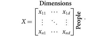
We denote the set of all possible matrices of size n ? d by X_n ∈ R+?^d and the set of all possible achievement matrices by X, such that X = U_n X_n.If X ∈ X_n, then matrix X contains achievements for n persons in d dimensions. Unless specified otherwise, whenever we refer to matrix X, we assume X ∈ X. The achievements of any person i in all d dimensions, which is row i of matrix X, are represented by the d-dimensional vector x_i. for all i = 1,..., n. The achievements in any dimension j for all n persons, which is column j of matrix X, are represented by the n-dimensional vector x._j for all j = 1,..., d.

In the unidimensional context, the d dimensions considered in matrix X ∈ X—which are typically assumed to be cardinal—can be meaningfully combined into a well-defined overall achievement or resource variable for each person i, which is denoted by x_i. One possibility, from a welfarist approach, would be to construct each person's welfare from her vector of achievements using a utility function x_i = u(x_i1,...,x_id).^[31] Another possibility is that each dimension j refers to a different source of income (labour income, rents, family allowances, etc.). Then, one can construct the total income level for each person i as the sum of the income level obtained from each source, that is x_i = ∑' 1 x_ij.

2.1.1 IDENTIFICATION OF THE INCOME POOR

Since Sen (1976), the measurement of poverty has been conceptualized as following two main steps: identification of who the poor are and aggregation of the information about poverty across society. In unidimensional space, the identification of who is poor is relatively straightforward: the poor are those whose overall achievement or resource variable falls below the poverty line z_u, where the subscript U simply signals that this is a poverty line used in the unidimensional space. Analogous to the construction of the resource variable, the poverty line can be obtained aggregating the minimum quantities or achievements zj considered necessary in each dimension. It is assumed that such quantities or levels are positive values, that is Zj ∈ R+₊.⁵ These minimum levels are collected in the d-dimensional vector z = (z₁,..., z_d).

If the overall achievement is the level of utility, a utility poverty line needs to be set as z_u = u(z₁,...,z_d).⁶ On the other hand, when the overall achievement is total income or

(say a rich one) is less important than some utility gain of another person (say a poor one).

⁴ Alkire and Foster (2011b) provide further discussion on uni- vs multidimensional approaches.

⁵ Theconcept ofthe poverty line dates to the late 1800s. Booth (1894,1903), Rowntree (1901), and Bowley and Burnett-Hurst (1915) wrote seminal studies based on surveys in some UK cities. As Rowntree writes, the poverty line represented the ‘minimum necessaries for the maintenance of merely physical efficiency’ (i.e. nutritional requirements) in monetary terms, plus certain minimum sums for clothing, fuel, and household sundries according to the family size (Townsend 1954: 131).

⁶ Axiomatic measures described in section 3.6.2 take this approach. total consumption expenditure, the poverty line is given by the estimated cost of the basic consumption basket z_u = ∑' 1 pj^zj—or some increment thereof.^[32]

Then, given the person's overall resource value or utility value and the poverty line, we can define the identification function as follows: ρ_u (x_i;z_u) = 1 identifies person i as poor if x_i < z_u, that is, whenever the resource or utility variable is below the poverty line, and ρ_u (x_i;z_u) = O identifies person i as non-poor if x_i ≥ z_u.

2.1.2 Aggregation of the income poor

In terms of aggregation, a variety of indices have been proposed.^[33] Among them, the FGT (1984) family of indices has been the most widely used measures of poverty by international organizations such as the World Bank and UN agencies, national governments, researchers, and practitioners.^[34]

For simplicity, we assume the unidimensional variable xi to be income. Building on previous poverty indices including Sen (1976) and Thon (1979), the FGT family of indices is based on the normalized income gap—called the ‘poverty gap' in the unidimensional poverty literature—which is defined as follows: given the income distribution x, one can obtain a censored income distribution x by replacing the values above the poverty line zu by the poverty line value zu itself and leaving the other values unchanged. Formally, x_i = x_i if x_i < z_u and x_i = z_u if x_i ≥ z_u. Then, the normalized income gap is given by

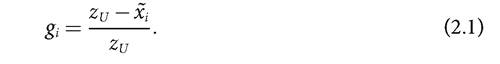
The normalized income gap of person i is her income shortfall expressed as a share of the poverty line. The income gap of those who are non-poor is equal to 0.^[35] The individual income gaps can be collected in an n-dimensional vector g^α = g,g%,...,g^). Eachg" element is the normalized poverty gap raised to the power α ≥ 0 and it can be interpreted as a measure of individual poverty where α is a ‘poverty aversion' parameter. The class of FGT measures is defined as P_α = ∑"_{= 1} gf /n, thus P_α can be interpreted as the average poverty in the population.

Within the FGT measures, three measures, associated with three different values of the parameter α, have been used most frequently. The deprivation vector g⁰, for α = 0, replaces each income below the poverty line with 1 and replaces non-poor incomes with 0. Its associated poverty measure P₀ = μ(g⁰) is called the headcount ratio, or the mean of the deprivation vector. It indicates the proportion of people who are poor, also frequently called the incidence of poverty.^[36] The normalized gap vector g¹, for α = 1, replaces each poor person's income with the normalized income gap and assigns 0 to the rest. Its associated measure P₁ = μ(g¹), the poverty gap measure, reflects the average depth of poverty across the society. The squared gap vector, g² for α = 2, replaces each poor person's income with the squared normalized income gap and assigns 0 to the rest. Its associated measure—the squared gap or distribution-sensitive FGT—is P₂ = μ(g²); it emphasizes the conditions of the poorest of the poor as Box 2.1 explains.

The FGT measures satisfy a number of properties, including a subgroup decomposabil­ity property that views overall poverty as a population-share weighted average of poverty levels in the different population subgroups.^[37] As noted by Sen (1976), the headcount ratio violates two intuitive principles: (1) monotonicity: if a poor person's resource level falls, poverty should rise and yet the headcount ratio remains unchanged; (2) transfer: poverty should fall if two poor persons' resource levels are brought closer together by a progressive transfer between them, and yet the headcount ratio may either remain unchanged or it can even go down. The poverty gap measure satisfies monotonicity, but not the transfer principle; the P2 measure satisfies both monotonicity and the transfer principle.^[38]

BOX 2.1 A NUMERICAL EXAMPLE OF THE FGT MEASURES

A simple example^[39] can clarify the method and these axioms, and will also prove useful in linking the Alkire and Foster methodology (fully described in Chapter 5) to its roots in the FGT class of poverty measures. Consider four persons whose incomes are summarized by vector x = (7,2,4,8) and the poverty line is z_u = 5.

The headcount ratio P₀: Consider first the case of a = 0. Each gap is replaced by a value of 1 if the person is poor and by a value of 0 if non-poor. The deprivation vector is given by: g⁰ = (0,1,1,0), indicating that the second and third persons in this distribution are poor. The mean of this vector—the P₀ measure—is one half: P₀ (x,z_U) = μ (g⁰) = 2/4 = 0.5, indicating that 50% of the population in this distribution is poor. Undoubtedly, it provides very useful information. However, as noted by Watts (1968) and Sen (1976), the headcount ratio does not provide information on the depth of poverty nor on its distribution among the poor. For example, if the third person became poorer, experiencing a decrease in her income so that the income distribution became x' = (7,2,3,8), the P₀ measure would still be one half; that is, it violates monotonicity. Also, if there was a progressive transfer between the two poor persons, so that the distribution was x" = (7,3,3,8), the P₀ measure would not change, violating the transfer principle. This has policy implications. If this was the official poverty measure, a government interested in maximizing the impact of resources on poverty reduction would have an incentive to allocate resources to the least poor, that is, those who were closest to the poverty line, leaving the lives of the poorest of the poor unchanged.

The poverty gap P₁ (or FGT-1): Here a = 1. Each gap is raised to the power a = 1, giving the proportion in which each poor person falls short of the poverty line and 0 if the person is non-poor. The normalized gap vector is given by g¹ = (0,3/5,1 /5,0). The P₁ measure is the mean of this vector. P₁ (x;z_u) = μ (g¹) = 4/20 indicates that the society would require an average of 20% of the poverty line for each person in the society to remove poverty. In fact, $4 is the overall amount needed in this case to lift both poor persons above the poverty line. Unlike the headcount ratio P₀, the P₁ measure is sensitive to the depth of poverty and satisfies monotonicity. If the income of the third person decreased so we had x = (7,2,3,8) the corresponding normalized gap vector would be g¹' = (0,3/5,2/5,0), so P₁ (x; z_U) = 5/20. Clearly, P₁ (x';z_υ^ > P₁ (x;z_u). Indeed, all measures with a > 0 satisfy monotonicity. However, a transfer to an extremely destitute person from a less poor person would not change P₁, since the decrease in one gap would be exactly compensated by the increase in the other. By being sensitive to the depth of poverty (i.e. satisfying monotonicity), the P₁ measure does make policymakers want to decrease the average depth of poverty as well as reduce the headcount. But because of its insensitivity to the distribution among the poor, P₁ does not provide incentives to target the very poorest, whereas the FGT-2 measure does.

The squared poverty gap P₂ (or FGT-2): When we set a = 2, each normalized gap is squared or raised to the power a = 2. The squared gap vector in this case is given by g² = (0,9/25,1/25,0). By squaring the gaps, bigger gaps receive higher weight. Note, for example, that while the gap of the second person (3/5) is three times bigger than the gap of the third person (1 /5), the squared gap of the second person (9/25) is nine times bigger than the gap of the third person (1/25). The mean of the g² vector—the P₂ measure—is P₂ (x;z_U) = μ (g²) = 10/100. The P₂ measure is sensitive to the depth of poverty: if the income of the third person decreases one unit such that x^, = (7,2,3,8), the squared gap vector becomes g² = (0,9/25,4/25,0), increasing the aggregate poverty level to P₂ (x';z_υ) = 13/100). It is also sensitive to the distribution among the poor: if there is a transfer of $1 from the third person to the second one, so x = (7,2,4,8) becomes x'' = (7,3,3,8), the squared gap vector becomes g² = (0,4/25,4/25,0), decreasing the aggregate poverty level to P₂ (x";z_u) = 8/100. Squaring the gaps has the effect of emphasizing the poorest poor and providing incentives to policymakers to address their situation urgently. All measures with a> 1 satisfy the transfer property.

1.2