Notation and Preliminaries for Multidimensional Poverty Measurement

We now extend the notation to the multidimensional context. We represent achievements as n ? d dimensional achievement matrix X, as in the unidimensional framework described in section 2.1.

We denote the set of all possible matrices of size n ? d by X_n ∈ R∙+?^d and the set of all possible achievement matrices by X, such that X = U_nX_n. If X ∈ X_n, then matrix X contains achievements for n persons and a fixed set of d dimensions. Unless specified otherwise, whenever we refer to matrix X, we assume X ∈ X. Thie achievements of any person i in all d dimensions, which is row i of matrix X, are represented by the d-dimensional vector x_i. for all i = 1,...,n. The achievements in any dimension j for all n persons, which is column j of matrix X, are represented by the n-dimensional vector X∙j for all j = 1,..., d.

In multidimensional analysis, each dimension may be assigned a weight or deprivation value based on its relative importance or priority.

1.2.1 identifyingdeprivations

A common first step in multidimensional poverty assessment in several of the meth­odologies reviewed in Chapter 3, as well as in the Alkire and Foster (2007, 2011a) methodology, requires defining a threshold in each dimension. Such a threshold is the minimum level someone needs to achieve in that dimension in order to be non-deprived. It is called the dimensional deprivation cutoff. When a person's achievement is strictly below the cutoff, she is considered deprived. We denote the deprivation cutoff in dimen­sion j by Zj; the deprivation cutoffs for all dimensions are collected in the d-dimensional vector z = (z₁,..., z_d). We denote all possible d-dimensional deprivation cutoff vectors by z ∈ R∙++∙ Any person i is considered deprived in dimension j if and only if x_ij < Zj.

For several measures reviewed in Chapter 3, and for the AF method, it will prove useful to express the data in terms of deprivations rather than achievements. From the achievement matrix X and the vector of deprivation cutoffs z, we obtain a deprivation matrix g⁰ (analogous to the deprivation vector in the unidimensional context) whose typical element g0 = ι whenever x_ij < z_j and g0 = o, otherwise, for all j = 1,..., d and for all i = 1,..., n. In other words, if person i is deprived in dimension j, then the person is assigned a deprivation status of 1, and 0 otherwise. Thus, matrix g⁰ (X) represents the deprivation status of all n persons in all d dimensions in matrix X.

On certain occasions, it will be useful to use the deprivation-cutoff censored achieve­ment matrix X which is obtained from the corresponding achievement matrix X in X, replacing the non-deprived achievements by the corresponding deprivation cutoff and leaving the rest unchanged. We denote the ij^th element of X by x_ij. Then, formally, x_ij = x_ij if x_ij < zj, and X_ij = zj otherwise. In this way, all achievements greater than or equal to the deprivation cutoffs are ignored in the censored achievement matrix.

When data are cardinally meaningful for all i = 1,..., n and all j = 1,..., d, and zj ∈ R₊₊, in other words, when all the achievements take non-negative values and the deprivation cutoffs take strictly positive values, one can construct dimensional gaps or shortfalls from the censored achievement matrix X as^[44]

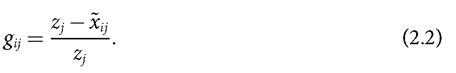
Each g_ij, or normalized gap, expresses the shortfall of person i in dimension; as a share of its deprivation cutoff. Naturally, the gaps of those whose achievement x_ij is above the corresponding dimensional deprivation cutoff z_j are equal to 0.

2.2.2 IDENTIFICATION AND AGGREGATION IN THE

Multidimensionalcase

Sen's (1976) steps of identification of the poor and aggregation also apply to the multi­dimensional case. It is clear that the identification of who is poor in the unidimensional case is relatively straightforward. The poverty line dichotomizes the population into the sets of poor and non-poor. In other words, in the unidimensional case, a person is poor if she is deprived. However, in the multidimensional context, the identification of the poor is more complex: the terms ‘deprived' and ‘poor' are no longer synonymous. A person who is deprived in any particular dimension may not necessarily be considered poor. An identification method, with an associated identification function, is used to define who is poor.

We denote the identification function by ρ, such that ρ (■) = 1 identifies person i as poor and ρ (■) = 0 identifies person i as non-poor. Analogous to the unidimensional case, we denote the number of multidimensionally poor people in a society by q and the set of poor persons in a society by Z, such that Z = {i∖ρ (■) = 1}. It could be the case that the identification method is based on some ‘exogenous' variable, in that it is a variable not included in achievement matrix X. For example, the exogenous variable could be being the beneficiary of some government programme or living in a specific geographic area.

There are many different ways of identifying the poor in the multidimensional context. A particularly prevalent set of methods consider the person's vector of achievements and corresponding deprivation cutoffs, such that ρ (x_i.;z) = 1 identifies person i as poor and ρ (x_i.; z) = O identifies person i as non-poor.^[45] Within this specification of the identification function, at least two approaches can be followed. An approach closely approximating unidimensional poverty is the ‘aggregate achievement approach', which consists of applying an aggregation function to the achievements across dimensions for each person to obtain an overall achievement value. The same aggregation function is also applied to the dimensional deprivation cutoffs to obtain an aggregate poverty line. As in the unidimensional case, a person is identified as poor when her overall achievement is below the aggregate poverty line. Another method, which we refer to as the ‘censored achievement approach', first applies deprivation cutoffs to identify whether a person is deprived or not in each dimension and then identifies a person by considering only the deprived achievements. The ‘counting approach' is one possible censored achievement approach, which identifies the poor according to the number (count) of deprivations they experience.

In counting identification methods, the criterion for identifying the poor can range from ‘union' to the ‘intersection'. The union criterion identifies a person as poor if the person is deprived in any dimension, whereas the intersection criterion identifies a person as poor only if she is deprived in all considered dimensions. In between these two extreme criteria there is room for intermediate criteria. Many counting-based measure­ment exercises since the mid-1970s have used an intermediate criterion (see Chapter 4). The AF methodology formally incorporated it into an axiomatic framework.^[46]

Once the identification method has been selected, the aggregation step requires selecting a poverty index, which summarizes the information about poverty across society. A poverty index is a function P : X ? z → R that converts the information contained in the achievement matrix X ∈ X and the deprivation cutoff vector z ∈ z into a real number. We denote a poverty index as P(X; z). An identification and an aggregation method that are used together constitute what we call a multidimensional poverty methodology, and we denote it as M = (ρ, P).

It will prove useful to introduce notation for two consistent sub-indices related to the overall poverty index P(X;z). Each of them offers information on different ‘slices' of the achievement matrix X as analysed by the corresponding multidimensional poverty methodology M = (ρ,P); that is, the consistent sub-indices are dependent on the selected identification and aggregation methods. One of these consistent sub-indices is the poverty level of a particular subgroup within the total population, denoted as P(X^t; z), where X^³ is the achievement matrix of this particular subgroup ˆ (which could be people of a particular ethnicity, for example) contained in matrix X. Visually, this consistent sub-index is based on a horizontal slice of the achievement matrix X (i.e. a set of rows).

The other consistent sub-index is a function of the post-identification dimensional deprivations, denoted as Pffx.pz), where, as stated above, vector x._j represents the achievements in dimension j for all n persons and z is the deprivation cutoff vector.^[47] This is precisely why the full vector of deprivation cutoffs z is an argument of the index and not just the particular deprivation cutoff zj. Recall that under some identification methods, it is possible to have some people who experience deprivations but are not identified as poor (for example, when a counting approach is used with an identification strategy that it is not union). In such cases, their deprivations will not be considered in the poverty measure and therefore will not be considered in this consistent sub-index either. In a visual way, this consistent sub-index is based on a vertical slice of the achievement matrixX (i.e. a column). These two consistent sub-indices will be used when introducing the different principles of multidimensional poverty measures in section 2.5.3.

As we shall see, although identification and aggregation have, since Sen (1976), usually been recognized as key steps in poverty measurement, some methods in the multidimensional context do not follow these steps. We will clarify this in Chapter 3.

2.2.3 Thejointdistribution

Throughout this book we will frequently refer to the joint distribution in contrast to the marginal distribution and we will also use the expression joint deprivations. The concept of a joint distribution comes from statistics where it can be represented using a joint cumulative distribution function.^[48] The relevance of the joint distribution in multidimensional analysis was articulated by Atkinson and Bourguignon (1982), who observed that multidimensional analysis was intrinsically different because there could be identical dimensional marginal distributions but differing degrees of interdependence between dimensions.^[49]

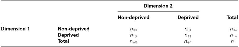
Table 2.1 Joint distribution of deprivation in two dimensions

In this book we treat the achievement matrix X as a representation of the joint distribution of achievements. Each row contains the (vector of) achievements of a given person in the different dimensions, and each column contains the (vector of) achievements in a given dimension across the population. From that matrix, considered with deprivation cutoffs, it is possible to obtain the proportion of the population who are simultaneously deprived in different subsets of d dimensions. In other words, it is possible to obtain the proportion of people who experience each possible profile of deprivations. This is visually clear in the deprivation matrixg⁰, which represents the joint distribution of deprivations. The higher-order matrices g¹ and g² obviously offer further information regarding the joint distribution of the depths of deprivations.

The importance of considering the joint distribution of achievements, which in turn enables us to look at joint deprivations, is best understood in contrast with the alternative of looking at the marginal distribution of achievements, and thus, the marginal deprivations. The marginal distribution is the distribution in one specific dimension without reference to any other dimension.^[50] The marginal distribution of dimension j is represented by the column vector xj. From the marginal distribution of each dimension, it is possible to obtain the proportion of the population deprived with respect to a particular deprivation cutoff. However, by looking at only the marginal distribution, one does not know who is simultaneously deprived in other dimensions.^[51]

Table 2.1 illustrates the relevance of the joint distribution in the basic case of n persons and two dimensions using a contingency table.

We denote the number of people deprived and non-deprived in the first dimension by n₁₊ and n₀₊, respectively; whereas, the number of people deprived and non-deprived in the second dimension are denoted by n₊₁ and n₊₀, respectively. These values correspond to the marginal distributions of both dimensions as depicted in the final row and final column of the table. They could equivalently be expressed as proportions of the total, in which case, for example, (n₁₊/n) would represent the proportion of people deprived (or the headcount ratio) in Dimension 1.

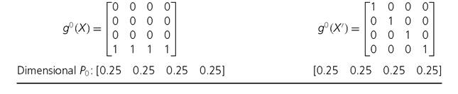
Table 2.2 Comparison of two joint distributions of deprivations in four dimensions

The marginal distributions, however, do not provide information about the joint distribution of deprivations, which is described in the four internal cells of the table. In particular, the number of people deprived in both dimensions is denoted by n₁₁, the number of people deprived in the first but not the second dimension is denoted by n₁₀, and the number of people deprived in the second and not in the first dimension is denoted by n₀₁. We know that n₁₁ people are deprived in both dimensions and the sum of n₁₁ + n₀₁ + n₁₀ is the number of people deprived in at least one dimension. These values correspond to the joint distribution of deprivations.

Consider now the case of four dimensions and four people, to see how valuable inform­ation can be added by the joint distribution. Table 2.2^[52] presents the deprivation matrix g⁰ of two hypothetical distributions, X and X'. Such a matrix presents joint distributions of deprivations in a compact way and is used regularly throughout this book.

In the table, the marginal distributions of each dimension's P₀ are identical in deprivation matrices g⁰ (X) and g⁰ (X'). Thus, the proportions of people deprived in each dimension are the same in the two distributions (25%). Yet, while, in distribution X, one person is deprived in all dimensions and three people experience zero deprivations, in distribution X', each of the four persons is deprived in exactly one dimension. In other words, although the marginal distributions are identical, the two joint distributions X and X' are very different. We understand that multiple deprivations that are simultaneously experienced are at the core of the concept of multidimensional poverty, and this is the reason why the consideration of the joint distribution is important. However, as we shall see, not all methodologies consider the joint distribution. In the next section, we introduce the notation for two methodologies of this type.

2.2.4 MARGINAL METHODS

Some of the methods for multidimensional poverty assessment introduced in Chapter 3 can be called marginal methods because they do not use information contained in the joint distribution of achievements. In other words, they ignore all information on links across dimensions. Following Alkire and Foster (2011b), a marginal method assigns the

same level of poverty to any two matrices that generate the same marginal distributions. In Table 2.2, a marginal method would assign the same poverty level to distribution X (four deprivations are experienced by one person) and distribution X' (each person experiences exactly one deprivation). That is, it would not be able to show whether the deprivations are spread evenly across the population or whether they are concentrated in an underclass of multiply deprived persons. Such marginal methods can also be linked to the order of aggregation while constructing poverty indices (Pattanaik et al. 2012). Specifically, a measure can be obtained by first aggregating achievements or deprivations across people (column-first) within each dimension and then aggregating across dimen­sions, or it can be obtained by first aggregating achievements or deprivations for each per­son (row-first) and then aggregating across people. Onlymeasures that follow the second order of aggregation (i.e. first across dimensions for each person and then across persons) reflect the joint distribution of deprivations (Alkire 2011: 61, figure 7). Measures that fol­low the first order of aggregation fall under marginal methods of poverty measurement.

Marginal methods also include cases where achievements for different dimensions are drawn from different data sources and/or from different reference groups within a population—as occurred, for example, in many indicators associated with the Millen­nium Development Goals. In this case, rather than having an n ? d dimensional matrixX of achievements, one may have a ‘collection' of vectors x^j ∈ R₊^j, representing the achieve­ments of n, people in dimension j for all j = 1,... d. Note that each x^j vector may refer to different sets of people such as children, adults, workers, or females, to mention a few.

Suppose, as before, that a deprivation cutoff Zj ∈ R₊₊ is defined. Then, we define a dimensional deprivation index Pj (x^j;Zj) for dimension j by Pj: R₊^j ? R₊₊ → R, which assesses the deprivation profile of n_j people in dimension j. The deprivation index might be simply the percentage of people who are deprived in this indicator or some other statistic such as child mortality rates. Note that deprivations are clearly identified in each dimension; however, because the underlying columns of dimensional achievements are not linked, no decision on who is to be considered multidimensionally poor can be made. This is a key difference between the dimensional deprivation index Pj (x^j; Zj) and the post-identification dimensional deprivation index Pj (x._j∙;z), which depends on the entire deprivation cutoff vector z (and not just Zj) and thus captures the joint distribution of deprivations (see section 2.2.2). Different dimensional deprivation indices Pj(x^j,Zj) can be considered in a set, constituting the ‘dashboard approach, or combined by some aggregation function, which is often called a ‘composite index' (Chapter 3).

2.2.5 USEFUL MATRIX AND VECTOR OPERATIONS

Throughout the book, we use specific vector and matrix operations. This section introduces the technical notation covering vectors and matrices.

We denote the transpose of any matrix X by X^tr where X^tr has the rows of matrix X converted into columns. Formally, if X ∈ Rⁿ ?^d and the ij^th element of X is written x_ij,

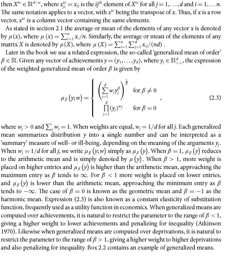
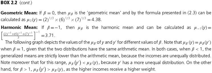
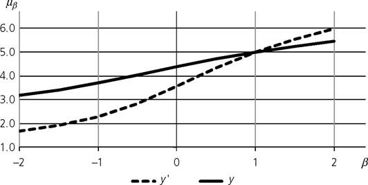
box 2.2 Exampleofgeneralizedmeans

Another matrix transformation that we use is replication. A matrix is a replication of another matrix if it can be obtained by duplicating the rows of the original matrix a finite number of times. Suppose the rows of matrix Y are replicated γ number of times, where γ ∈ N∖{1}. Then the corresponding replication matrix is denoted by rep(Y;γ). This notation may be used for replication of any vector y: rep(y; γ). We do not consider column replication, as we consider a fixed set of dimensions.

We also use three types of matrices associated with particular operations: a permuta­tion matrix, a diagonal matrix, and a bistochastic matrix. A permutation matrix, denoted by ∏, is a square matrix with one element in each row and each column equal to 1 and the rest of the elements equal to 0. Thus the elements in every row and every column sum to one. We eliminate the special case when a permutation matrix is an ‘identity matrix' with the diagonal elements equal to 1 and the rest equal to 0. What does a permutation matrix do? If any matrix Y is pre-multiplied by a permutation matrix, then the rows of matrix Y are shuffled without their elements being altered. Similarly, if any matrix Y is post-multiplied by a permutation matrix, then the columns of Y are shuffled without their elements being altered.

Example of Permutation Matrix: Let Y

Consider ∏

Then ΠY =

Thus, the rows of Y are merely swapped. Similarly, consider

swapped their positions. The first column did not change its position because the first diagonal element in ∏ is equal to one.

A diagonal matrix, denoted by Λ, is a square matrix whose diagonal elements are not necessarily equal to 0 but all off-diagonal elements are equal to 0. Let us denote the ij^th element of Λ by A_ij-. Then, A_ij- = 0 for all i = j. For our purposes, we require the diagonal elements of a diagonal matrix to be strictly positive or A_ii > 0. What is the use of a diagonal matrix? If any matrix Y is post-multiplied by a diagonal matrix, then the elements in each column are changed in the same proportion. Note that different columns may be multiplied by different factors.

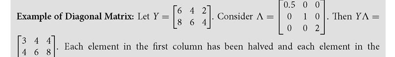
third column has been doubled. However, the second column did not change because the corresponding element of Λ is equal to one.

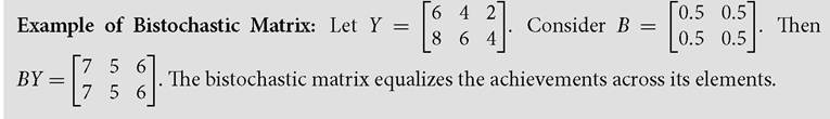
A bistochastic matrix, denoted by B, is a square matrix in which the elements in each row and each column sum to one. If the ij^th element of B is denoted by B_ij, then ∑_iB_ij = 1 for all j and ∑_jB_ij = 1 for all i. Why do we require a bistochastic matrix? If a matrix is pre-multiplied by a bistochastic matrix, then the variability across the elements of each column is reduced while their average or mean is preserved. Note that if a diagonal element in a bistochastic matrix is equal to one, the achievement vector of the corresponding person remains unaffected. If the bistochastic matrix is a permutation matrix or an identity matrix, then the variability remains unchanged.

2.3