Scales of Measurement: Ordinal and Cardinal Data
An important element of the framework in multidimensional poverty measurement relates to the scales of measurement of the indicators used. Scales of measurement are key because they affect the kind of meaningful operations that can be performed with indicators.
In fact, as we will observe, certain types of indicators may not allow a number of operations and thus cannot be used to generate certain poverty measures.What does scale of measurement refer to exactly? Following Roberts (1979) and Sarle (1995), we define a scale of measurement to be a particular way of assigning numbers or symbols to assess certain aspects of the empirical world, such that the relationships of these numbers or symbols replicate or represent certain observed relations between the aspects being measured. There are different classifications of scales of measurement. In this book, we follow the classification introduced by Stevens (1946) and discussed in Roberts (1979). Stevens' classification is consistent with Sen (1970,1973), which analysed the implications of scales of measurement for welfare economics, distributional analysis, and poverty measurement, and it has largely stood the test of time.[53]
Stevens' (1946) classification relies on four key concepts: assignment rules, admissible transformations, permissible statistics, and meaningful statements. First, the defining feature of a scale is the rule or basic empirical operation that is followed for assigning numerals, as elaborated below. Second, each scale has an associated set of admissible mathematical transformations such that the scale is preserved. That is, if a scale is obtained from another under an admissible transformation, the rule under the transformed scale is the same as under the original one. Third, a permissible statistic refers to a statistical operation that when applied to a scale, produces the same result as when it is applied to the (admissibly) transformed scale.
While the word ‘permissible' may sound rather strong, it is justifiable under the premise that ‘one should only make assertions that are invariant under admissible transformations of scale' (Marcus-Roberts and Roberts 1987: 384).[54]° Fourth, a statement is called meaningful if it remains unchanged when all scales in the statement are transformed by admissible transformations (Marcus-Roberts and Roberts 1987: 384).[55]Stevens (1946) considered four basic empirical operations or rules that define four types of scales: equality, rank order, equality of intervals, and equality of ratios. Following them, he defined four main types of scales: nominal, ordinal, interval, and ratio. Stevens' classification is not exhaustive. For example, it only applies to scales that take real values and which are regular.[56] Also, note that alternative terms are sometimes used for some of Stevens' types. For example, nominal scales are sometimes referred to as categorical scales.
Table 2.3 lists the scale types mentioned above from ‘weakest' to ‘strongest' in the sense that interval and ratio scales contain much more information than ordinal or nominal scales. The column that presents the rule defining each scale type is cumulative in the sense that a rule listed for a particular scale must be applicable to the scales in rows preceding it. The column that lists the permissible statistics is also cumulative in the
Table 2.3 Stevens' classification of scales of measurement
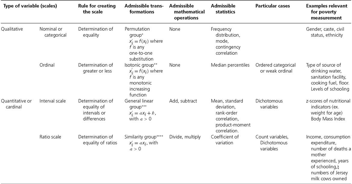
Source: Stevens (1946). The columns on 'Particular cases' and 'Examples' have been added by the authors.
[1] A permutation group here refers to the composition of permutations that can be performed with elements of a group.
[1] An isotonic group here refers to the set of transformations which preserve order.
[1] A general linear group here refers to the set of linear transformations (with the specifications stated above).
[1] A similarity group here refers to the set of ratio transformations (with the specifications stated above).
⅛ Note that years of schooling may also be interpreted in an ordinal sense, depending on the meaning attached.
same sense. In contrast, the column that lists the admissible transformations goes from general to particular: the particular operation listed in a row is included in the operation listed above.
We now introduce each scale ‘type’. The scale pertains to an indicator used to measure dimension j. The term ‘indicator j denotes the indicator of dimension j. Achievements in indicator j across the population are represented by vector xij ∈ R”, where xij is the achievement of person i in the jth indicator.
Indicator j is said to be nominal or categorical if the scale is based on mutually exclusive categories, which are not necessarily ordered. Nominal variables are frequently called categorical variables. The rule or basic empirical operation behind this type of scale is the determination of equality among observations. A nominal scale is ‘the most unrestricted assignment of numerals. The numerals are used only as labels or type numbers, and words or letters would serve as well’ (Stevens 1946: 678). That is, numbers assigned to the various achievement levels in this domain are simply placeholders.
Stevens introduces two common types of nominal variables. One uses ‘numbering’ for identification, such as the identification number of each household in a survey or the line number of individuals living within a household. The other uses numbering for a classification, such that all members of a social group (ethnic, caste, religion, gender, or age) or geographical region (rural/urban areas, states, or provinces) are assigned the same number. The first type of nominal variable is simply a particular case of the second. There is a wide range of admissible transformations for this type of scale. In fact, any transformation that substitutes or permutes values between groups, that is, any one-to-one substitution function f such that xi = f (xj for all i, will leave the scale form invariant.
Given that in a nominal variable the different categories do not have an order, neither arithmetic operations nor logical operations (aside from equality) are applicable. In terms of relevant statistics, if the nominal variable is simply an identifier, then only the number of categories is a relevant statistic; if the nominal variable contains several cases in each category, then the mode and contingency methods can be implemented, as can hypotheses tests regarding the distribution of cases among the classes (Stevens 1946: 678-9).
Indicator j is said to be ordinal if the order matters but not the differences between values. The rule or basic empirical operation behind this type of scale is the determination of a rank order. Categories can be ordered in terms of ‘greater’, ‘less’, or ‘equal’ (or ‘better’, ‘worse’, ‘preferred’, ‘not preferred’). Admissible transformations consist of any order-preserving transformation, that is, any strictly monotonic increasing function f such that xij =f (xij) for all i, as these will leave the scale form invariant. Thus, admissible transformations include logarithmic operation, square root of the values (non-negative), linear transformations, and adding a constant or multiplying by another (positive) constant. Examples of ordinal scales are preference orderings over various categories, or subjective rankings. Given that the true intervals between the scale points are unknown, arithmetic operations are meaningless (because results will change with a change of scale), but logical operations are possible. For example, we can assert that someone reporting a health level of four feels ‘better’ than someone reporting a health level of ‘three’, who in turn feels better than a ‘two’, but we cannot assert whether the difference between level three and four is the same as the difference between level two and three. Nevertheless, some statistics are applicable to ordinal variables, namely, the number of cases, contingency tables, the mode, median, and percentiles.[54] Statistics such as mean and standard deviation cannot be used.
Clearly, an ordinal variable is a nominal variable but the converse is not true. Ordinal and nominal (or categorical) variables are also sometimes referred to as qualitative variables.Unordered categorical variables—such as eye colour—are not relevant for the construction of poverty measures. Relevant categorical variables are those that can be exhaustively and non-trivially partitioned into at least two sets according to some exogenous condition, and in which those sets can be arranged in a complete ordering. There will be fewer sets than there are categorical responses, or else the original variable would already have been ordinal. If a set contains multiple elements, it may not be possible to rank those elements against one another. Hence the resulting construction would be a ‘semi-order’ (Luce 1956) or ‘quasi-order’ (Sen 1973). Additionally, it may be possible to distinguish set(s) that are considered to be adequate achievements from those that are inadequate, forming a ‘weak order’ that is, some pairs of responses can be ranked as ‘preferred to’ and some others cannot be ranked.[55] For example, because it is difficult to assess whether it is better to have access to a public tap than to a borehole or a protected well as sources of drinkable water, the Millennium Development Goal indicator considers all three of them to be adequate sources of drinkable water (unrankable). Similarly, while one cannot rank access to an unprotected spring versus access to rainwater, both sources are considered inadequate by MDG standards. A variable thus constructed is often called an ‘ordered categorical’; we might also call the variables obtained as a weak order of categories in a nominal variable, a ‘weak-ordinal’ variable. Admissible transformations of weak ordinal variables include any transformations that partition the categorical variables into the relevant sets (safe water sources) in the same order; any apparent ordering of elements within the relevant sets can vary freely.
Indicator j is said to be of interval scale if the rule or basic empirical operation behind its scale is the determination of the equality of intervals or differences.
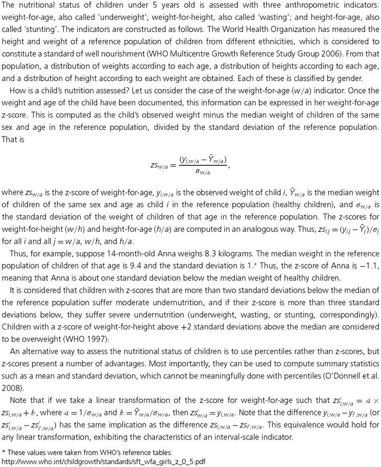
Importantly, interval scales do not have a predefined zero point. The admissible transformations of interval scale consist of the linear transformation x!ij = axij + b (with a > 0), as this preserves the differences between categories. While the difference between two values of an interval-scale variable is meaningful, the ratios are not. The most cited example in this literature refers to two temperature scales: Celsius (°C) and Fahrenheit (°F). While the difference between 15°C and 20°C is the same as the difference between 20°C and 25°C, one cannot say that 20°C is twice as hot as 10°Ń because 0°Ń does not mean ‘no temperature’. That is, the Celsius scale (and Fahrenheit scale) lack a natural zero. Also, the difference between 150C and 20°C and between 20°Ń and 25°Ń is also precisely the same if measured in Fahrenheit (59°F and 68°F vs 68°F and 77°F) although the value of the difference is nine rather than five degrees. An interval scale allows addition and subtraction and the computation of most statistics, namely, number of cases, mode, contingency correlations, median, percentiles, mean, standard deviation, rank-order correlation, and product-moment correlation, but it is not meaningful to compute the coefficient of variation or any other ‘relative’ measure.In multidimensional poverty measurement, one indicator that is usually of interest is the z-score of under 5-year-old children’s nutritional achievement. We consider a nutritional z-score to be of interval-scale type. Box 2.3 provides a more detailed explanation of how to compute z-scores. Z-scores range from negative to positive values, spaced in (the reference population’s) standard deviation units, and the zero value means that the child’s nutritional achievement is at the median of what is considered a healthy population.
Indicator j is said to be of ratio scale if the rule or basic empirical operation behind its scale is the determination of equality of ratios. Such a rule requires the scale to have a ‘natural zero’: namely the value 0 means ‘no quantity’ of that indicator. In other words, the value 0 is the absolute lowest value of the variable. Admissible transformations of interval-scale variables consist of functions such as x,j = axj (with a > 0), as this preserves the ratio differences. Examples of ratio-scale variables are age, height, weight, and temperature in Kelvin, as 0° Kelvin means ‘no temperature’, 200 pounds is twice as much as 100 pounds, sixty years as thirty years, and so on. Ratio-scale variables allow statements such as ‘a value is twice as large as another’, and they allow any type of mathematical operation, as well as the computation of any statistic (number of cases, mode, contingency correlations, median, percentiles, mean, standard deviation, rank-order correlation, product-moment correlation, and coefficient of variation). Interval- and ratio-scale variables constitute what are commonly referred to as cardinal variables.
It is interesting to observe that in the order presented, from nominal to ratio scales, the admissible transformations become more restricted but the meaningful statistics become more unrestricted, ‘suggesting that in some sense the data values carry more information’ (Velleman and Wilkinson 1993: 66). Stevens (1959: 24) provided an insightful example of how measurement can progress from weaker to stronger scales. Early humans probably could only distinguish between cold and warm and thus used a nominal scale. Later, degrees of warmer and colder had been introduced and so the use of an ordinal scale gained prominence. The introduction of thermometers led to the use of an interval scale. Finally, the development of thermodynamics led to the ratio scale of temperature by introducing the Kelvin scale.
BOX 2.3 CHILDREN'S NUTRITIONAL Z-SCORES
Having introduced the scales of measurement, it is worth making a few clarifications regarding other frequently mentioned types of indicators. First, Stevens' classification makes no reference to continuous versus discrete variables, for example. Continuous variables can take any value on the real line within a range. Discrete variables, in contrast, can only take a finite or countably infinite number of values.[56] Ordinal variables are discrete variables, but cardinal ones (interval and ratio scale) can be either discrete or continuous.[57] Second, note that count variables such as counts of publications, number of children in a household, or number of chickens, are particular cases of ratio-scale variables (Stevens 1946), such that the only admissible transformation is the identity function, i.e. a = 1. Roberts (1979) refers to the counting scale type as an absolute scale.
Third, dichotomous (also called binary) variables can be of different scales, depending on the meaning of their categories. When the two values simply refer to unordered, mutually exclusive categories, such as being male or female, the variable is of nominal scale. When there is an order between the categories, such as being deprived or not in a specific dimension, the variable is cardinal. If the two values refer to having or lacking the same thing, such as a fully functional method for wood smoke ventilation, the variable maybe interpreted as of ratio scale.[58]
Fourth, the reader may wonder where do Likert scales—introduced by Likert (1932) and often used in social sciences—fit? Likert scales are obtained from responses to a set of (carefully phrased) statements to which each respondent expresses her level of agreement on a scale such as one to five: strongly disagree, disagree, neutral, agree, or strongly agree. Each statement and its responses are known as a Likert item. A Likert scale is obtained by summing or averaging the responses to each item so that a score is acquired for each person. Likert scales are frequently treated as interval scales, under the assumption (at times empirically verified) that there is an equal distance between categories (Brown 2011; Norman 2010). Thus, descriptive statistics (like means and standard deviations) and inferential statistics (like correlation coefficients, factor analysis, and analysis of variance) are regularly implemented with Likert scales. However, this has been criticized as being ‘illegitimate to infer that the intensity of feeling between “strongly disagree” and “disagree” is equivalent to the intensity of feeling between other consecutive categories on the Likert scale' (Cohen et al. 2000, cited in Jamieson 2004: 1217). Thus, there is ongoing disagreement about whether Likert scales should be treated as ordinal scales (Pett 1997; Hansen 2003; Jamieson 2004). Often empirical psychometric tests are performed to ‘verify' whether the assumption that the scale can be treated as cardinal holds for a particular dataset.
Stevens' (1946) landmark work sparked a body of literature on measurement theory, which raised strong warnings regarding the applicability of statistics to different scales, including Stevens (1951,1959), Luce (1959), and Andrews et al. (1981). This engendered an extensive and ongoing debate across literatures from psychology to statistics. Some social scientists and statisticians consider that although, in theory, certain statistics such as the mean and standard deviations are inappropriate for ordinal data, they can still be ‘fruitfully' applied if the problem in question and data structure (and comparability, if relevant) have been tested and seem to warrant assumptions that they can be treated as interval scale. The arguments in favour of this position are interestingly articulated by Velleman and Wilkinson (1993). For example, it is stated that ‘the meaningfulness of a statistical analysis depends on the questions it is designed to answer' (Lord 1953; Guttman 1977), that in the end ‘every knowledge is based on some approximation' (Tukey 1961), and that ‘„.if science was restricted to probably meaningful statements it could not proceed' (Velleman and Wilkinson 1993). Another argument is that parametric methods are highly robust to violation of assumptions and thus can be implemented with ordinal data (Norman 2010). Although we acknowledge this ongoing debate, in what follows we do endorse the requirement of meaningfulness—as defined above—in order to compute statistics or mathematical measures in each scale type; hence, we limit the operations with ordinal data to those that cohere with its definition and point out deviations from this.
As this section suggests, the indicators' scale and the analysts' considered response to scales of measurement must be articulated before selecting a methodology to measure and assess multidimensional poverty. In Chapter 3, we clarify whether each method surveyed can be used with ordinal data. In general, when an indicator is of ratio scale, such as income, consumption, or expenditure (all expressed in monetary units), arithmetic operations with elements of the scale are permissible. Thus, it is meaningful to compute the normalized deprivation gaps as defined in Expression (2.2). When all considered indicators are of ratio scale, multidimensional poverty measures based on normalized deprivation gaps can be used. If the indicator is of interval scale, gaps may be redefined appropriately. When indicators are ordinal, measures based on normalized deprivation gaps are meaningless because results would vary under different admissible transformations of the indicators' scales. The Adjusted Headcount Ratio presented in Chapters 5-10 can be meaningfully implemented using ordinal indicators, provided that issues of comparability are addressed, as we will now clarify.
1.3