Robustness Analysis
In monetary poverty measures, the parameters include (a) the set of indicators (components of income or consumption); (b) the price vectors used to construct the aggregate as well as any adjustments such as for inflation or urban/rural price differentials; (c) the poverty line; and (d) equivalence scales (if applied).
The parameters that influence the multidimensional poverty estimates and poverty comparisons based on the Adjusted Headcount Ratio are (i) the set of indicators (denoted by subscript j = 1,..., d); (ii) the set of deprivation cutoffs (denoted by vector z); (iii) the set of weights or deprivation values (denoted by vector w); and (iv) the poverty cutoff (denoted by k). A change in these parameters may affect the overall poverty estimate or comparisons across regions or countries.This section introduces tools that can be used to test the robustness of pairwise comparisons as well as the robustness of overall rankings with respect to the initial choice of the parameters. We first introduce a tool to test the robustness of pairwise comparisons with respect to the choice of the poverty cutoff. This tool tests an extreme form of robustness, borrowing from the concept of stochastic dominance in the single-dimensional context (section 3.3.1).[216] When dominance conditions are satisfied, the strongest possible results are obtained. However, as dominance conditions are highly stringent and dominance tests may not hold for a large number of the pairwise comparisons, we present additional tools for assessing the robustness of country rankings using the correlation between different rankings. This second set of tools can be used with changes in any of the other parameters too, namely, weights, indicators, and deprivation cutoffs.
8.1.1 DOMINANCE ANALYSIS FOR CHANGES IN THE POVERTY CUTOFF
Although measurement design begins with the selection of indicators, weights, and deprivation cutoffs, we begin our robustness analysis by assessing dominance with respect to changes in the poverty cutoff, which is applied to the weighted deprivation scores constructed using other parameters.
We do this because as in the unidimensional context, it is the poverty cutoff that finally identifies who is poor, thereby defining the ‘headcount ratio' and effectively setting the level of poverty. It is arguably most visibly debated.3 We have introduced the concept of stochastic dominance in the uni- and multidimensional context in section 3.3.1. This part of the chapter builds on that concept and technique, focusing primarily on first-order stochastic dominance (FSD) and showing how it can be applied to identify any unambiguous comparisons with respect to the poverty cutoff for our two most widely used poverty measures—Adjusted
Let us now explain how we can apply this concept for unanimous pairwise comparisons using M0 and H between any two distributions of deprivation scores across the population. For a given deprivation cutoff vector z and a given weighting vector w, the FSD tool can be used to evaluate the sensitivity of any pairwise comparison to varying poverty cutoff k. Following the notation introduced in Chapter 2, we denote the (uncensored) deprivation score vector by c. Note that an element of c denotes the deprivation score and a larger deprivation score implies a lower level of well-being.
The FSD tool can be applied in two different ways: one is to convert deprivations into attainments by transforming the deprivation score vector c into an attainment score 
5 This is also variously known as survival function or reliability function in other branches of studies.
6 Technically, M0 for poverty cutoff k can be expressed as M0 = fkFc(x)dx + kFc (k). In our example, Area I is computed as fk Fc(x)dx and Area II as kFc(k).
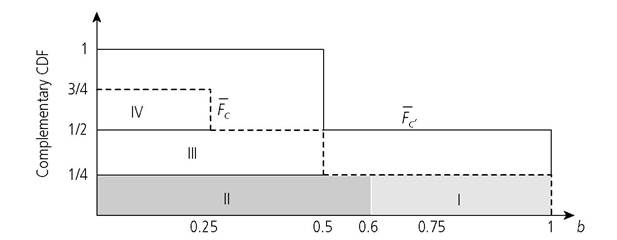
Figure 8.1.
Complementary CDFs and poverty dominance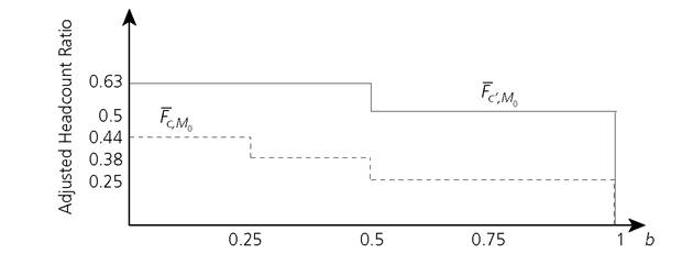
Figure 8.2. The Adjusted Headcount Ratio dominance curves
Therefore, when the CCDFs of two distributions cross—i.e. there is not first-order (H) dominance—it is worth testing M0 dominance between pairs of distributions, which we refer to as pairwise comparisons from now on, using the M0 curves. Batana (2013) has used the M0 curves for the purpose of robustness analysis while comparing multidimensional poverty among women in fourteen African countries.
The dominance requirement for all possible poverty cutoffs may be an excessively stringent requirement. Practically, one may seek to verify the unambiguity of comparison with respect to a limited variation in the poverty cutoff, which can be referred to as restricted dominance analysis. For example, when making international comparisons in terms of the MPI, Alkire and Santos (2010, 2014) tested the robustness of pairwise comparisons for all poverty cutoffs k ∈ [0.2, 0.4], in addition to the poverty cutoff of
k = 1/3. In this case, if the restricted FSD holds between any two distributions, then dominance holds for the relevant range of poverty cutoffs for both H and M0.
8.1.2 RANK ROBUSTNESS ANALYSIS
In situations where dominance tests are too stringent, we may explore a milder form of robustness. It assesses the extent to which a ranking, that is, an ordering of more than two entities obtained under a specific set of parameters' values, is preserved when the value of some parameter is modified. How should we assess the robustness of a ranking? One first intuitive measure is to compute the percentage of pairwise comparisons that are robust to changes in parameters—that is, the proportion of pairwise comparisons that have the same ordering. As we shall see in section 8.3, whenever poverty computations are performed using a survey, the statistical inference tools need to be incorporated into the robustness analysis.
Another useful way to assess the robustness of a ranking is by computing a rank correlation coefficient between the original ranking of entities and the alternative rankings (i.e. those obtained with alternative parameters' values). There are various choices for a rank correlation coefficient. The two most commonly used rank correlation coefficients are the Spearman rank correlation coefficient (Rρ) and the Kendall rank
7 In this book, we only focus on bivariate rank correlation coefficients, but there are various methods to measure multivariate rank concordance that we do not cover. For such examples, see Boland and Proschan (1988), Joe (1990), and Kendall and Gibbons (1990). For an application of some ofthe multivariate concordance methods to examine multivariate concordance of MPI rankings, see Alkire et al. (2010). lowest across the two specifications. In terms of the previous approach, 0% of the pairwise comparisons are robust to changes in one or more parameters' values.
The Spearman rank correlation coefficient can be expressed as
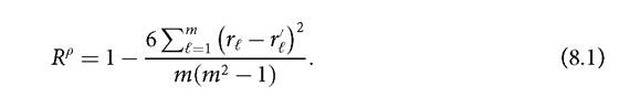
Intuitively, for the Spearman rank correlation coefficient, the square of the difference in the two ranks for each subgroup is computed and an average is taken across all subgroups. The Rρ is bounded between — 1 and +1. The lowest value of — 1 is obtained when two rankings are perfectly negatively associated with each other, whereas the largest value of +1 is obtained when two rankings are perfectly positively associated with each other.
non-robust pairwise comparison. The Rτ is the difference in the number of concordant and discordant pairs divided by the total number of pairwise comparisons.
The Kendall rank correlation coefficient can be expressed as
Like Rρ, Rτ also lies between — 1 and +1. The lowest value of — 1 is obtained when two rankings are perfectly negatively associated with each other, whereas the largest value of+1 is obtained when two rankings are perfectly positively associated with each other. Although both Rρ and Rτ are used to assess rank robustness, the Kendall rank correlation coefficient has an intuitive interpretation. Suppose the Kendall Tau correlation coefficient is 0.90, from equation (8.2), it can be deduced that this means that 95% of the pairwise comparisons are concordant (i.e. robust) and only 5% are discordant. Equations (8.1) and (8.2) are based on the assumption that there are no ties in the rankings. In other words, both expressions are applicable when no two entities have equal values. When there are ties, Kendall (1970) offers two adjustments in the denominator of both rank correlation coefficients (Rρ and Rτ) to correct for tied ranks; these adjusted Kendall coefficients are commonly known as tau-b and tau-c.
Let us present one empirical illustration showing how rank robustness tools may be used in practice. The first illustration presents the correlation between 2011 MPI rankings across 109 countries and the rankings for three alternative weighting vectors (Alkire et al. 2011). The MPI attaches equal weights across three dimensions: health, education, and standard of living. However, it is hard to argue with perfect confidence that the
Table 8.1 Correlation among country ranks for different weights
Equal weights
| Alternative Weights 1 | Spearman | 0.979 |
| Kendall | 0.893 | |
| Alternative Weights 2 | Spearman | 0.987 |
| Kendall | 0.918 | |
| Alternative Weights 3 | Spearman | 0.985 |
| Kendall | 0.904 |
Note: The computations of the Spearman and Kendall coefficients in the table have been adjusted for ties.
For the exact formulation of tie-adjusted coefficients, see Kendall and Gibbons (1990).
initial weight is the correct choice. Therefore, three alternative weighting schemes were considered. The first alternative assigns a 50% weight to the health dimension and then a 25% weight to each of the other two dimensions. Similarly, the second alternative assigns a 50% weight to the education dimension and then distributes the rest of the weight equally across the other two dimensions. The third alternative specification attaches a 50% weight to the standard of living dimension and then 25% weights to each of the other two dimensions. Thus, we now have four different rankings of 109 countries, each involving 5,356 pairwise comparisons. Table 8.1 presents the rank correlation coefficient Rρ and Rτ between the initial ranking and the ranking for each alternative specification. It can be seen that the Spearman coefficient is around 0.98 for all three alternatives. The Kendall coefficient is around 0.9 for each of the three cases, implying that around 80% of the comparisons are concordant in each case.
The same type of analysis has been done to changes in other parameters' values, such as the indicators used and deprivation cutoffs (Alkire and Santos 2014).
8.2