Statistical Inference
The last section showed how the robustness of claims made using the Adjusted Headcount Ratio and its partial and consistent sub-indices maybe assessed. Such assessments apply to changes in a country's performance over time, comparisons between different countries, and comparisons of different population subgroups within a country.
Most frequently, the indices are estimated from sample surveys with the objective of estimating the unknown population parameters as accurately as possible. A sample survey, unlike a census that covers the entire population, consists of a representative fraction of the population.8 Different sample surveys, even when conducted at the same time and despite having the same design, would most likely provide a different set of estimates for the8 Various sampling methods, such as simple random sampling, systematic sampling, stratified sampling, and proportional sampling, are used to conduct a sampling survey.
same population parameters. Thus, it is crucial to compute a measure of confidence or reliability for each estimate from a sample survey. This is done by computing the standard deviation of an estimate. The standard deviation of an estimate is referred to as its standard error. The lower the magnitude of a standard error, the larger the reliability of the corresponding estimate. Standard errors are key for hypothesis testing and for the construction of confidence intervals, both of which are very helpful for robustness analysis and more generally for drawing policy conclusions. In what follows we briefly explain each of these statistical terms.
8.2.1 STANDARD ERRORS
There are different approaches to estimating standard errors. Two approaches are commonly followed:
• Analytical Approach: Formulas that provide either the exact or the asymptotic approximation of the standard error and thus confidence intervals.[217]
• Resampling Approach: Standard errors and the confidence intervals maybe computed through the bootstrap or similar techniques (as performed for the global MPI in Alkire and Santos 2014).
The Appendix to this chapter presents the formulas for computing standard errors with the analytical approach depending on the survey design.
The analytical approach is based on two assumptions. Such assumptions are based on the premise that the sample surveys used for estimating the population parameters are significantly smaller in size compared to the population size under consideration.[218] For example, the sample size of the Demographic and Health Survey of India in 2006 was only 0.04% of the Indian population. The first assumption is that the samples are drawn from a population that is infinitely large, so that even the finite population under study is a sample of an infinitely large superpopulation. This philosophical assumption is based on the superpopulation approach, which is different from the finite population approach (for further discussion see Deaton 1997). A finite population approach requires that a finite population correction factor should be used to deflate the standard error if the sample size is large relative to the population. However, if the sample size is significantly smaller than the finite population size, the finite population correction factor is approximately equal to one. In this case, the standard errors based on both approaches are almost the same.
The second assumption is that we treat each sample as drawn from the population with replacement. The practical motivation behind the assumption is the size of the sample survey compared to the population. The sample surveys are commonly conducted without replacement because, once a household is visited and interviewed, the same household is not visited again on purpose. When samples are drawn with replacement, the observations are independent of each other. However, if the samples are drawn without replacement, then the samples are not independent of each other. It can be shown that in the absence of multistage sampling, a sampling without replacements needs a Finite Population Correction (FPC) factor for computing the sampling variance.
The FPC factor is of the order 1 — n/n, where n is the sample size and n is the size of the population. The use of an FPC factor allows us to get a better estimate of the true population variance. However, when the sample size is small with respect to the population, i.e. n/n → 0, the use of an FPC factor will not make much difference to the estimation of the sampling variance as the FPC factor is closer to one (Duclos and Araar 2006: 276). These assumptions would be required in order to justify our assumption that each sample is independently and identically distributed.We now illustrate relevant methods using the Adjusted Headcount Ratio (M0) denoting its sample estimate by M0 and standard error of the estimate by se^. However, the methods are equally applicable to inferences for the multidimensional headcount ratio, the intensity, and the censored headcount ratios as long the standard errors are appropriately computed, as outlined in the Appendix of this chapter.
8.2.2 CONFIDENCE INTERVALS
A confidence interval is a type of interval estimate of a parameter. The probability that a confidence interval contains the parameter is called the confidence level. A significance level that is used is the complement of the confidence level. Let us denote the significance level[219] by ω, which by definition ranges between 0 and 100%. The level of confidence is (1 — ω) percent. Thus, for a given estimate, if one wants to be 95% confident about the range within which the true population parameter lies, then the significance level is 5%. Similarly, if one wants to be 99% confident, then the significance level is 1%.
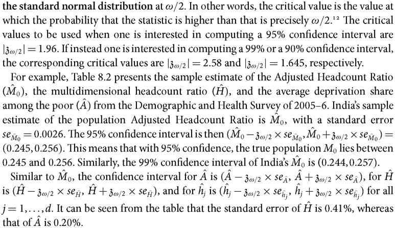
By the central limit theorem, we can say that the difference between the population parameter and the corresponding sample average divided by the standard error approximates the standard normal distribution (i.e. the normal distribution with a mean of 0 and a standard deviation of 1). Using the standard normal distribution, one can determine the critical value associated with that significance level, which is given by the inverse of
Table 8.2 Confidence intervals for M0, H, and A
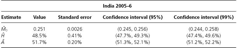
Source: Alkire and Seth (2013b, 2015)
8.2.3 HYPOTHESIS TESTS
Confidence intervals are useful for judging the statistical reliability of a point estimate when the population parameter is unknown.
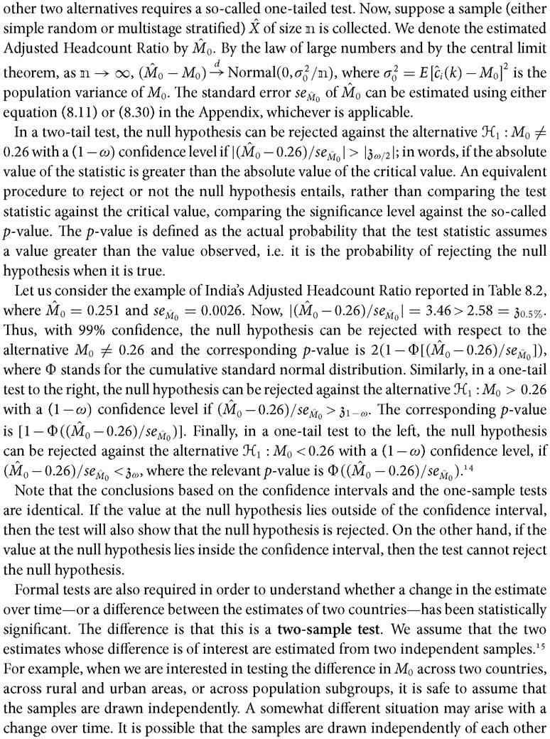
However, suppose that, somehow, we have a hypothesis about what the population parameter is. For example, suppose the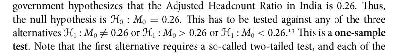
[1] The critical values will follow a Student-t distribution if the population standard deviation is estimated or if the sample size is small.
[1] We present the tests for country-level estimates but they are equally applicable to other population subgroups. Also, we only present the tests in terms of the X0 measure, but again they are also applicable to A, H, and hj for all j, and so we have chosen not to repeat the results.
14 See Bennett and Mitra (2013) for an exposition of hypothesis testing of M0 and other AF partial sub-indices using a minimum p-value approach.
15 See chapters 14 and 16 of Duclos and Araar (2006) for further discussion of non-independent samples for panel data analysis.
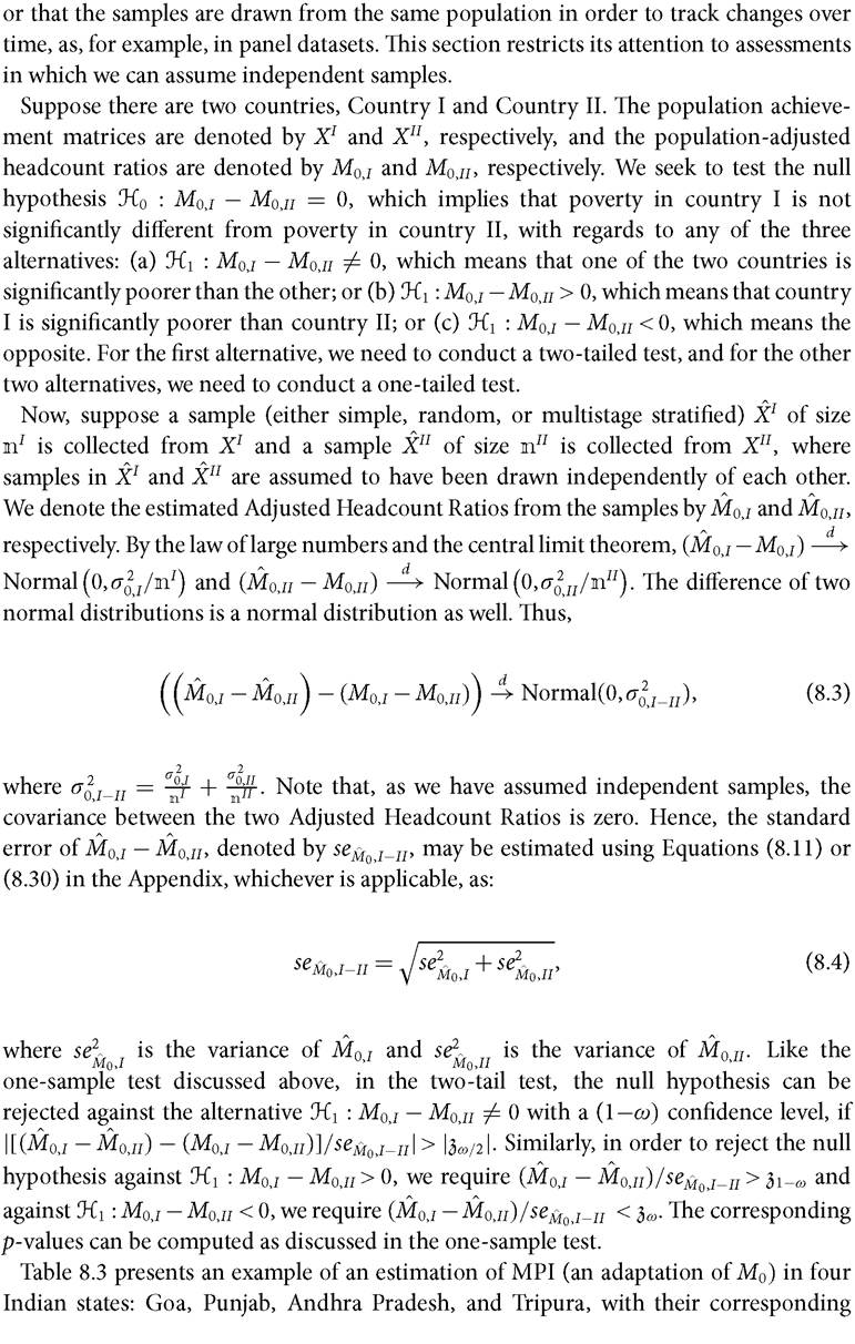
Table 8.3 Comparison of Indian states using standard errors
| States | MPI | Standard error | 95% Confidence interval | Difference | ||
| Lower bound | Upper bound | MPI | Statistically significant | |||
| Goa | 0.057 | 0.0062 | 0.045 | 0.069 | 0.031 | Yes |
| Punjab | 0.088 | 0.0078 | 0.073 | 0.103 | ||
| Andhra Pradesh | 0.194 | 0.0093 | 0.176 | 0.212 | 0.032 | No |
| Tripura | 0.226 | 0.0162 | 0.195 | 0.258 | ||
Source: Alkire and Seth (2013b)
standard errors, confidence intervals, and hypothesis tests.[220] These results are computed from the Demographic and Health Survey of India for the years 2005-6.
In the table we can see that the MPI point estimate for Goa is 0.057, and with 95% confidence, we can say that the MPI estimate of Goa lies somewhere between 0.045 and 0.069. Similarly, we can say with 95% confidence that Punjab's MPI is not larger than 0.103 and no less than 0.073, although the point estimate of MPI is 0.088. We can also state, after doing the corresponding hypothesis test, that Punjab is significantly poorer than Goa. However, we cannot draw the same kind of conclusion for the comparison between Andhra Pradesh and Tripura, although the difference between the MPI estimates of these two states (0.032) is similar to the difference between Goa and Punjab.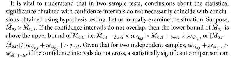
be made. However, if the confidence intervals overlap, it does not necessarily mean that the comparison is not statistically significant at the same level of significance. It is thus essential to conduct statistical tests on differences when the confidence intervals overlap.
8.3
More on the topic Statistical Inference:
- CONTENTS
- Conditional probability as fundamental
- BACKGROUND AND DEFINITIONS
- Probability spaces
- Adolfo Garcia de la Sienra. A Structuralist Theory of Economics. New York, USA: Routledge,2019. — 235 p., 2019
- Recapitulating the Interlocking, Amplifying, and Inhibiting Institutions of Violence