Robustness Analysis with Statistical Inference

In practice, the robustness analyses discussed in section 8.1 are typically performed with estimates from sample surveys. In at least two cases, it is necessary to combine the robustness analyses with the statistical inference tools just described.

The dominance analysis presented in section 8.1.1 assesses dominance between two CCDFs or two M₀ curves in order to conclude whether a pairwise ordering is robust to the choice of all poverty cutoffs. But it is also crucial to examine if the pairwise dominance of the CCDFs or M₀ curves are statistically significant. For two entities in a pairwise order­ing, one should perform one-tailed hypothesis tests of the difference in the two M₀ estim­ates for each possible k value, as described in section 8.2.3. This will determine whether the two countries' poverty estimates are not significantly different or whether one is sig­nificantly poorer than the other regardless of the poverty cutoff.^[221] One may also construct confidence interval curves around each CCDF curve (or M₀ curve) and examine whether two corresponding confidence interval curves overlap or not, in order to conclude dominance. More specifically, if the lower confidence interval curve of a unit does not overlap with the upper confidence interval curve of another unit, then one may conclude that statistically significant dominance holds between two entities. However, as explained at the end of section 8.2.3, no conclusion on statistical significance can be made when the confidence intervals overlap. Thus a hypothesis test for dominance should be preferred.^[222]

This method also applies to the other type of robustness analysis presented in section 8.1.2, in the sense that one can implement this analysis to a ranking of entities and report the proportion of robust pairwise comparisons across the different k values.

As Alkire and Santos observe (2014: 260), the number of robust pairwise comparisons may be expressed in two ways. One may report the proportion of the total possible pairwise comparisons that are robust. A somewhat more precise option is to express it as a proportion of the number of significant pairwise comparisons in the baseline measure, because a pairwise comparison that was not significant in the baseline M0 cannot, by definition, be a robust pairwise comparison.

To interpret results meaningfully, it can be helpful to observe that the proportion of robust pairwise comparisons of alternative M₀ specifications is influenced by the number of possible pairwise comparisons, the number of significant pairwise comparisons in the baseline distribution, and the number of alternative parameter specifications. Interpret­ation of the percentage of robust pairwise comparisons in light of these three factors illuminates the degree to which the poverty estimates and the policy recommendations they generate are valid across alternative plausible design specifications.

Alkire and Santos (2014) perform both types of robustness analysis with the global MPI (2010 estimates) for every possible pair of countries with respect to (a) a restricted range of k values, namely, 20% to 40%; (b) four alternative sets of plausible weights; and (c) subgroup-level MPI values.^[223] The country rankings seem highly robust to alternative parameters' specifications.^[224]

Chapter 9 further develops the techniques of multidimensional poverty measurement and analysis. Specifically, we present techniques for analysing poverty over time (with and without panel data) and for exploring distributional issues such as inequality among the poor.

Appendix: Methods for Computing Standard Errors

This appendix provides a technical outline of how standard errors maybe computed. We first present the analytical approach and then the bootstrap method using the notation in Method I, presented in Box 5.7. For the multidimensional and censored headcount ratios, we use the notation in Box 5.4. The M₀ and its partial and consistent sub-indices are written as

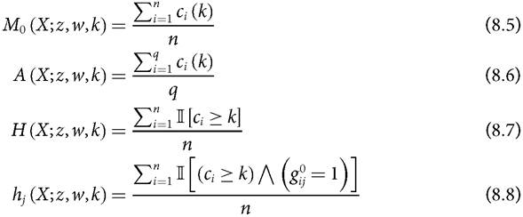
Note that ∕∖ is the logical ‘and' operator. The standard errors of the subgroups' M₀s and partial and consistent sub-indices may be computed in the same way and so we only outline the standard errors of equations (8.5)-(8.8).

Simple Random Sampling with Analytical Approach

Suppose n samples have been collected through simple random sampling from the population. We denote the dataset by X and its j^th element by X_ij for all i = 1,..., n and j = 1,..., d. We denote the deprivation status score for X_ij by g_i0. For statistical inferences, our analysis focuses on the censored deprivation scores. The score, defined at the population level, becomes a random variable while performing statistical inference. We assume that a random sample (of size n) of censored deprivation scores {c₁ (k),..., c_n (k)} is a sequence of independently and identically distributed random variables with an

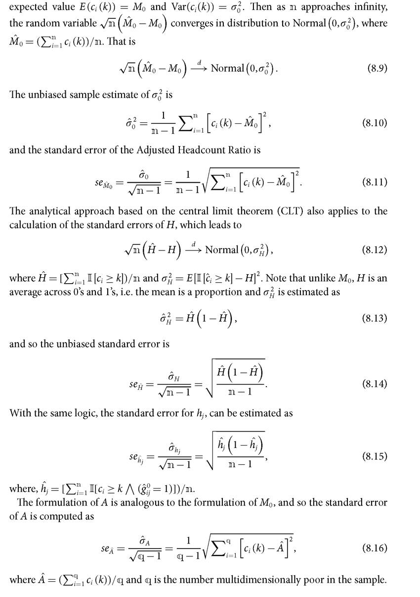
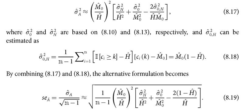
Note that if the number of multidimensionally poor is extremely low, the sample size for estimating seχ may not be large enough. Thiis may affect the precision of seχ using (8.16). It may then be accurate to treat A as a ratio of M₀ and H for computing se^. By the Taylor series expansion (see the discussion in Casella and Berger 1990, 240-245), A can be approximated as A ≈ M₀∕H and σA can be estimated as

Stratified Sampling with an Analytical Approach

We next discuss the estimation of standard errors when samples are collected through two-stage stratification.²¹ Using information on the population characteristics, the population is partitioned into several strata.

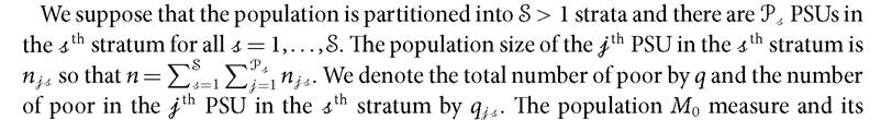
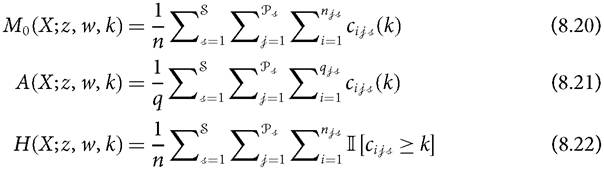
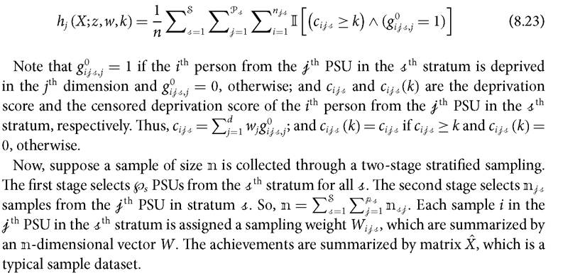
partial and consistent sub-indices are presented in (8.20)-(8.23) with the same notation for the identity function as in (8.5)-(8.8).

²¹ Appendix D of Seth (2013) gives an example of standard error estimation for one-stage sample stratification in the multidimensional welfare framework; for consumption/expenditure see Deaton (1997).

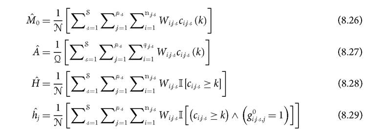
In order to estimate the measure from the sample, first, the total population and the total number of poor should be estimated from the sample. We denote the estimates of the population n by N and the estimate of the poor population q by Q. Then,

The sample estimates of the population averages in (8.20)-(8.23) are presented in (8.26)-(8.29).

As each sample estimate is a ratio of two estimators, their standard errors are approxim­ated using (8.17) and using equations (1.31) and (1.63) in Deaton (1997). The standard error for M₀ in (8.26) is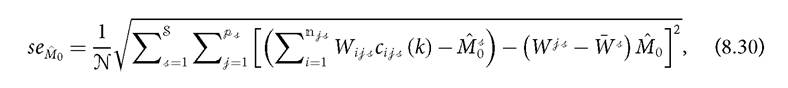

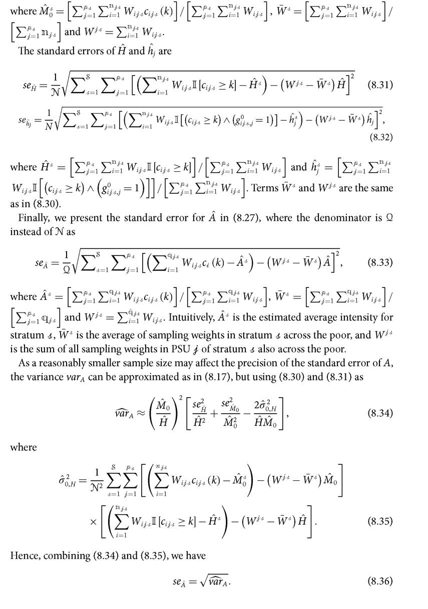
Note that the analytical standard errors and confidence intervals may not serve too well when the sample sizes are small or when the estimates are too close to the natural upper or lower bounds.^[225] In these cases, resampling methods, such as bootstrap, may be more suitable for computing standard errors and confidence intervals.

The Bootstrap Method

An alternative approach for statistical inference is the ‘bootstrap, which is a data-based simulation method for assessing statistical accuracy. Introduced in 1979, it provides an estimate of the sampling distribution of a given statistic θ, such as the standard error, by resampling from the original sample (cf. Efron 1979; Efron and Tibshirani 1993). It has certain advantages over the analytical approach. First, the inference on summary statistics does not rely on the CLT as the analytical approach. In particular, for a reasonably small sample size, standard errors/confidence intervals computed through the CLT-based asymptotic approximation may be inaccurate. Second, the bootstrap can automatically take into account the natural bounds of the measure. Confidence intervals using the analytical approach can lie outside natural bounds, which can be prevented when the bootstrap resampling distribution of the statistic is directly used.

Third, the computation of standard errors may become complex when the estimator and its standard error have a complicated form or have a no-closed expression. These types of complexities are common both in the context of statistical inference of inequality or poverty measurement and in tests where comparisons of group in­equality or poverty (across gender or region) are of particular interest (Biewen 2002). Although the delta-method can handle these analytical standard errors from stochastic dependencies, when the number of time periods or groups increases, computing the standard errors analytically can easily become cumbersome (cf. Cowell 1989; Nygard and Sandstrom 1989). In practice, Monte Carlo evidence suggests that bootstrap methods are preferred for these analyses and shows that the simplest bootstrap pro­cedure achieves the same accuracy as the delta-method (Biewen 2002; Davidson and Flachaire 2007). In development economics, the bootstrap has been used to draw statistical inferences for poverty and inequality measurement (Mills and Zandvakili 1997; Biewen 2002).

Here we briefly illustrate the use of the bootstrap for computing standard errors. Read­ers interested in using the bootstrap for confidence interval estimation and hypothesis testing can refer to Efron and Tibshirani (1993), chapters 12 and 16, respectively.

The bootstrap algorithm can be described as a resampling technique, which is conducted B number of times by generating a random artificial sample each time, with

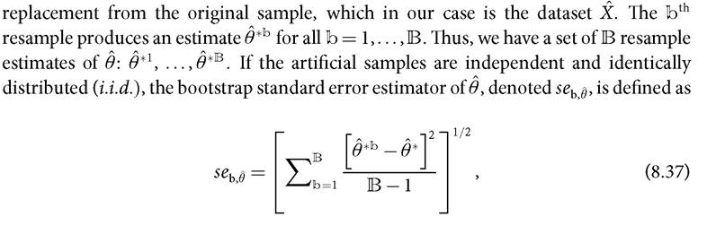
where θ*' stands for the arithmetic mean over the artificial samples. Even if the artificial sample is drawn from a more complex but known sampling framework, the bootstrap standard error can be easily estimated from standard formulas (c.f. Efron 1979, Efron and Tibshirani 1993). If the resampling is conducted on an empirical distribution of a given dataset X, then it is referred to as a non-parametric bootstrap. In this case, each observation is sampled (with replacement) from the empirical distribution, with probability inversely proportional to the original sample size. However, the resampling can also be selected from a known distribution chosen on an empirical or theoretical basis. In this case, it is referred to as a parametric bootstrap.

BOX 8.1 BOOTSTRAP STANDARD ERRORS OF THE ADJUSTED HEADCOUNT RATIO AND ITS COMPONENTS

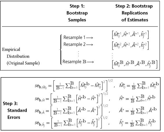
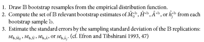
Box 8.1 illustrates the use of the bootstrap for computing standard errors for M₀ and its partial and consistent sub-indices. In this case, the statistic θ comprises M₀, H, A, and hj. Thus, the estimate θ includes M₀, H, A, or hj. To obtain the bootstrap standard errors, we need to pursue the following steps.

We have already discussed that the bootstrap approach has certain advantages— especially that it does not rely on the central limit theorem. Although the non-parametric bootstrap approach does not depend on any parametric assumptions, it does involve certain choices. The first is the number of replications. Indeed a larger number of replications increases the precision of the estimates, but is costly in terms of time. There are different approaches for selecting the appropriate number of replications (see Poi 2004 for example). The second involves the choice of the bootstrap sample size being selected from the original sample. The third involves the choice of the resampling method. The bootstrap sample size in Efron's traditional bootstrap is equal to the number of observations in the original sample, but the use of smaller sample sizes has also been studied (for further theoretical discussions; see Swanepoel (1986) and Chung and Lee (2001)).

9