The Set of Partial and Consistent Sub-Indices of the Adjusted Headcount Ratio
The Adjusted Headcount Ratio condenses a lot of information. It can be unpacked to compare not only the levels of poverty but also the dimensional composition of poverty across countries, for example, as well as within countries by ethnic group, urban and rural location, and other key household and community characteristics.
This is why we sometimes describe M0 as a high-resolution lens on poverty: it can be used as an analytical tool to identify precisely who is poor and how they are poor. This section presents the partial indices and consistent sub-indices that serve to elucidate multidimensional poverty for policy purposes.5.5.1 INCIDENCE AND INTENSITY OF POVERTY
We have already shown in section 5.3 that the M0 measure is the product of two very informative partial indices: the multidimensional headcount ratio—or incidence of poverty (H)—and the average deprivation share across the poor—or the average intensity of poverty (A). Both are relevant and informative, and it is useful to present them both when reporting M0. In Box 5.5, we present an example to show that two societies may have the same Adjusted Headcount Ratios but very different levels of incidence and intensity.
BOX 5.5 SAME M BUT DIFFERENT COMPOSITION OF INCIDENCE AND INTENSITY
BOX 5.5 (cont.)
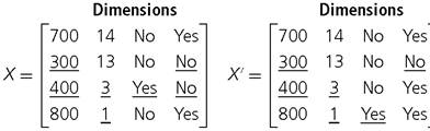
and the deprivation cutoff vector z = (500, 5, Not malnourished, Has access to improved sanitation). The corresponding deprivation matrices are denoted as follows.
The deprivation score column vectors (not shown) are c = (0,0.5,1,0.25) and c = (0,0.5,0.5,0.5), respectively. Clearly, the second and the third person are identified as poor in X and the second, third, and fourth persons are identified as poor in X'.
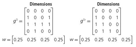
The corresponding censored deprivation matrices are as follows.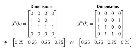
The breakdown of M0 into H and A can provide useful policy insights. A policymaker who is interested in reducing overall poverty when poverty is assessed by the Adjusted Headcount Ratio may do so in different ways. If M0 is reduced by focusing on the poor who have a lower intensity of poverty, then there will be a large reduction in H. But there may not be a large reduction in the average intensity (A). On the other hand, if the policies are directed towards the poorest of the poor, then an overall reduction in M0 may be accomplished by a larger reduction in A instead of H. Thus, while monitoring poverty reduction, it is possible to see how overall poverty has been reduced.
It should be noted that H and A are also partial indices of the other Mα measures. Additionally, these other measures, such as M1 and M2, also have other informative partial indices, discussed in section 5.1.
5.5.2 SUBGROUP DECOMPOSITION
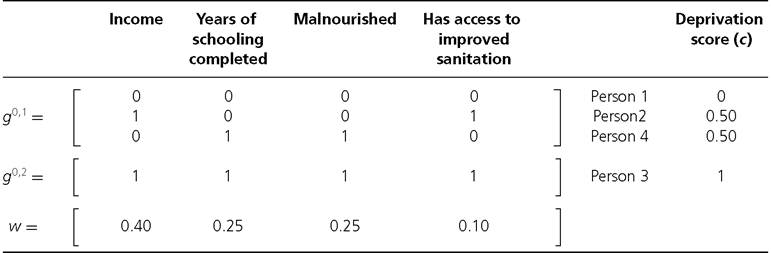
In developing multidimensional methods, we would not want to lose the useful properties that the unidimensional methods have successfully employed over the years. Prime among them is population subgroup decomposability, which, as stated in section 2.5.3, posits that overall poverty is a population-share weighted sum of subgroup poverty levels. This property has proved to be of great use in analysing poverty by regions, by ethnic groups, and by other subgroups defined in a variety of ways.[170] The M0 measure, as well as the other Mα measures, satisfies the population subgroup decomposability property, a property that is directly inherited from the FGT class of indices (Foster, Greer, and Thorbecke 1984).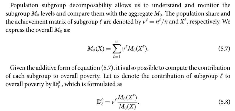
Note that the contribution of subgroup f to overall poverty depends both on the level of poverty in subgroup f and on the population share of the subgroup.
Whenever the contribution to poverty of a region or some other group greatly exceeds its population share, this suggests that there is a seriously unequal distribution of poverty in the country, with some regions or groups bearing a disproportionate share of poverty. Clearly, the sum of the contributions of all groups needs to be 100%.[171]5.5.2.1 Subgroup Decompositions of the Adjusted Headcount Ratio (M0)
Let us consider the example of the hypothetical society presented in Box 5.1 and show how the contribution of subgroups to the overall Adjusted Headcount Ratio is computed. For this example, let us assume a certain weighting structure and a certain poverty cutoff to identify who among these four persons is poor. We assume that a 40% weight is
Table 5.1 Achievement matrices of subgroups in the hypothetical society
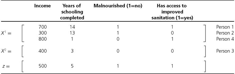
Table 5.2 (Censored) deprivation matrices of the subgroups
attached to income, a 25% weight is attached to years of education, a 25% weight is attached to undernourishment, and the remaining 10% weight is attached to the access to improved sanitation. Thus, the weight vector is w = (0.40,0.25,0.25,0.10). Weidentify a person as poor if the person is deprived in 40% or more of weighted indicators, that is, k = 0.40.
For subgroup decomposition, we divide the entire population in X into two subgroups. Subgroup 1 consists of three persons, whereas Subgroup 2 consists of only one person as presented in Table 5.1. Note that the person in Subgroup 2 is deprived in all dimensions. We denote the achievement matrix of Subgroup 1 by X1 and that of Subgroup 2 by X2.
The deprivation matrices and deprivation scores of the two subgroups are presented in Table 5.2. Person 1 is not deprived in any dimension and so has a deprivation score of 0.
Person 2 is deprived in two dimensions: income and access to improved sanitation, and so the deprivation score is 0.5. Similarly, the deprivation score of Person 4 is 0.5 and Person 3,s is 1. Now, for k = 0.4, Person 2 and Person 4 are poor in Subgroup 1 and Person 3 is poor in Subgroup 2. In both subgroups, those who are deprived are identified as poor, and so there is no scope for censoring. The censored deprivation matrices for both groups are, in this particular case, the corresponding deprivation matrices.
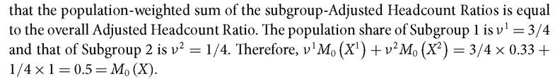
Note that the Adjusted Headcount Ratio in Subgroup 2 is more than three times larger than the Adjusted Headcount Ratio of Subgroup 1. Does this mean that the contribution of Subgroup 2 is also more than three times as large as the contribution of Subgroup 1? No it does not. Recall that the contribution of a subgroup to overall poverty depends on the population share of that subgroup as well. For our example, the contribution of Subgroup 1 to the overall Adjusted Headcount Ratio is D0 = (3/4 ? 0.33)/0.5 = 0.5 or 50%. The contribution of Subgroup 2 to the overall headcount ratio is D° = (1/4 ? 1)/0.50 = 0.5 or 50%. It is worth noting that, in this case, the population Subgroup 2 does bear a disproportionate load of poverty since, despite being only 25% of the total population, it contributes 50% of overall poverty. Because population shares affect interpretation, tables showing subgroup decompositions can benefit from including population shares for each subgroup, as well as poverty figures.
5.5.3 Dimensionalbreakdown
As discussed in section 2.5, a multidimensional poverty measure that satisfies the dimensional breakdown property can be expressed as a weighted sum of the dimensional deprivations after identification. The M0 satisfies the dimensional breakdown property and thus can also be expressed as a weighted sum of post-identification dimensional deprivations, which in the particular case of M0 we refer to as the censored headcount ratios.
Why is this property useful? This property allows one to analyse the composition of multidimensional poverty. For example, Alkire and Foster (2011a), after decomposing overall poverty in the United States by ethnic group, break the poverty within those groups down by dimensions and examine how different ethnic groups have different dimensional deprivations, i.e. different poverty compositions.
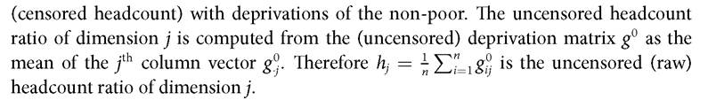
The censored headcount ratio of a dimension is defined as the percentage of the population who are multidimensionally poor and simultaneously deprived in that dimension. Formally, we denote the jth column of the censored deprivation matrix g0 (k) as g0 (k) and mean of the column for that chosen dimension as hj (k) = 1V n_ 1 g0 (k). Then hj (k) is simply the censored headcount ratio of dimension j. What is the interpretation of hj (k)? The censored headcount ratio hj (k) is the proportion of the population that are identified as poor (ci ≥ k) and are deprived in dimension j.
The additive structure of the M0 measure allows it to be expressed as a weighted sum of the censored headcount ratios, where the weight on dimension j is Wj, the relative weight assigned to that dimension. We have already seen in expression (5.3) that

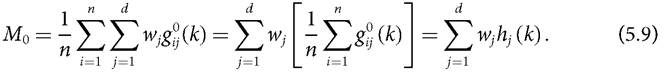
Analyses based on the censored headcount ratios can be complemented in an interesting way by considering the percentage contribution of each dimension to overall poverty. The censored headcount ratio shows the extent of deprivations among the poor but not the relative value of the dimensions. Two dimensions may have the same censored headcount ratios but very different contributions to overall poverty. This is because the contribution not only depends on the censored headcount ratio but also on the weight or 
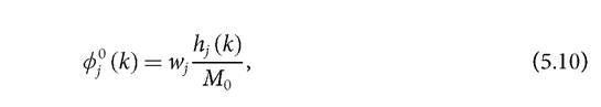 for each j = 1,..., d.
The uncensored (raw) headcount ratio of a dimension is defined as the proportion of the population that are deprived in that dimension. It aggregates deprivations of the poor
The censored headcount ratio generally differs from the uncensored headcount ratio except when the identification criterion used is union. In this case, a person is identified as poor if the person is deprived in any dimension, so no deprivations are censored. Thus, the censored and uncensored headcount ratios are identical.
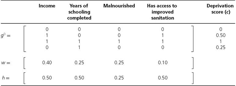
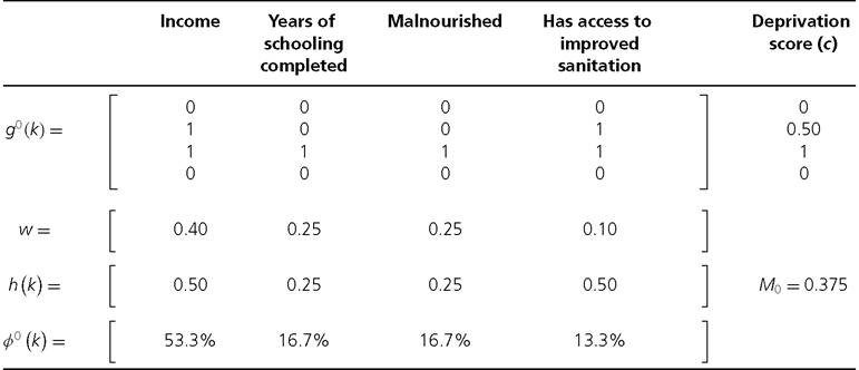
Table 5.3 Deprivation matrix of the hypothetical society
5.5.3.1 The Censored and Uncensored Headcount Ratios and Percentage Contributions
Using a hypothetical illustration, we now show how the uncensored headcount ratios and the censored headcount ratios are computed and then calculate the contribution of each dimension to the Adjusted Headcount Ratio. Let us consider the same achievement matrix and weight vector as was in the previous subsection, which consists of four persons and four dimensions.
of the nutritional status dimension is 25%, and of access to improved sanitation is 50%. The uncensored headcount ratios (summarized by vector h) are reported in the bottom row of the table.
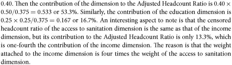
Next, we show how to compute the censored headcount ratio. We identify a person as poor if the person is deprived in 40% of weighted indicators, i.e. k = 0.4. Using the identification function we construct the censored deprivation matrix, presented in Table 5.4. Note that we censor the deprivations of Person 4 and replace them by O even though Person 4 is deprived in the education dimension. Why do we do this? We do so because the deprivation score of Person 4 is only 0.25, which is less than the poverty cutoff of k = 0.4, and hence Person 4 is not poor. It can be easily verified that the M0 measure is 0.375. 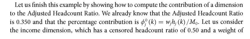
Table 5.4 Censored deprivation matrix of the hypothetical society
5.6