A Case Study: The Global Multidimensional Poverty Index (MPI)
Now that we have learned how to compute the Adjusted Headcount Ratio and its partial indices, we provide an example showing one prominent implementation of the M0 measure: the global Multidimensional Poverty Index (MPI).
The global MPI was developed by Alkire and Santos (2010) with UNDP's Human Development Report Office and has been reported annually in the Human Development Report since 2010.[173] The index consists of ten indicators grouped into three dimensions, as outlined in Table 5.5.Note that the index uses nested weights. The weights are distributed such that each dimension reported in the first column receives an equal weight of 1/3 and the weight is equally divided among indicators within each dimension (note the distinction in terms here between indicator and dimension). Thus, each education and health indicator
Table 5.5 Dimensions, indicators, deprivation cutoffs, and weights of the global MPI
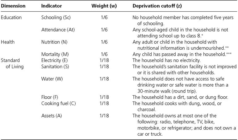
Source: Alkire and Santos (2010, 2014); cf. Alkire, Roche, Santos, and Seth (2011) and Alkire, Conconi, and Roche (2013)
* If a household has no school-aged children, the household is treated as non-deprived.
** An adult with a Body Mass Index below 18.5 m/kg2 is considered undernourished. A child is considered undernourished if his or her body weight, adjusted for age, is more than two standard deviations below the median of the reference population.
*** If no person in a household has been asked this information, the household is treated as non-deprived.
receives larger weights than the standard of living indicators. The weights for each indicator are reported in the third column. The deprivation cutoffs are outlined in the final column. Any person living in a household who fails to meet the deprivation cutoff is identified as deprived in that indicator.
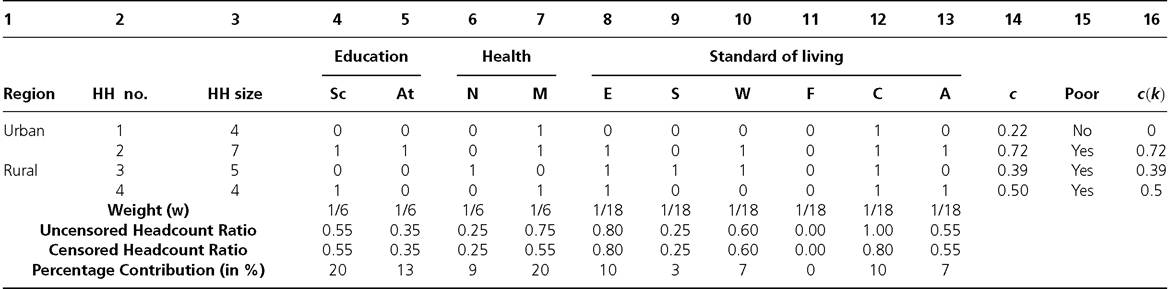
An abbreviation has been assigned to each indicator in the second column that will be useful for the presentations in the next table.Table 5.6 presents a hypothetical example of people living in four households, which will help explain how the MPI is constructed. The first two households live in urban areas and the third and the fourth households live in rural areas. In this illustration, the households are not of equal size. The household sizes are reported in the third column of the table. The deprivation matrix (g0) is presented in columns 4 through 13. Following the standard notation, a 1 indicates that a household is deprived in the corresponding indicator and 0 indicates that the household is not deprived in that indicator. For example, the first household is only deprived in mortality (M) and cooking fuel (C), whereas the fourth household is deprived in five indicators: schooling (Sc), mortality (M), electricity (E), cooking fuel (C), and asset ownership (A).
Let us first show how the deprivation score (ci) of each person is computed. Note that in this example, all persons within a household are assigned the same deprivation score, which is the weighted sum of deprivations that the household faces. For example, the
Table 5.6 The deprivation matrix and the identification of the poor
deprivation score of each person in the first household is
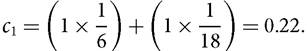
The deprivation scores are reported in column 14. The deprivation scores of the second, third, and fourth households are 0.72, 0.39, and 0.50, respectively. Thus, the second household has the largest deprivation score and the first household has the lowest deprivation score.
In the computation of the global MPI, a person is identified as poor if the person's deprivation score is equal to 1/3 or higher.
It is evident from column 14 that the first household's deprivation score is less than 1/3, whereas the three other households' deprivation scores are larger than 1/3. Thus, all persons in the first household are identified as non-poor, whereas all other persons in the last three households are identified as multidimensionally poor. Column 15 classifies the households as multidimensionally poor or not. The multidimensional headcount ratio or the incidence of poverty (H) is (hint: use the household size)
So 80% of the population are poor. Note that we have already discussed that the multidimensional headcount ratio (H) does not satisfy the dimensional monotonicity property, and so it does not change if any of the three poor households become deprived in an additional dimension. This limitation is overcome by the Adjusted Headcount Ratio (M0), which is called the MPI in this example. The censored deprivation scores are reported in column 16, where the deprivation score of the non-poor household has been censored by replacing the score by 0. The MPI is the mean of the censored deprivation score vector and can be computed using expression (5.3) as (hint: use the household size)

One may be also interested in knowing how poor the poor people are, or the intensity of multidimensional poverty. The intensity of poverty can be computed as
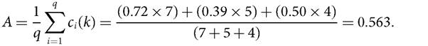
So, on average, poor people are deprived in 56.3% of the weighted indicators. It can be easily verified that the MPI is the product of the incidence of poverty and the intensity of poverty, i.e. MPI = H ? A = 0.8 ? 0.563 = 0.450.
Let us now show how the subgroup decomposition property maybe used to understand the contribution of subgroups to overall multidimensional poverty.
Using the same process as above, the MPI, H, and A can be computed for each population subgroup. The MPI of the two urban households is 0.46, which can be obtained either by summing the censored deprivation scores weighted by the population share of each household or as a product of H = 0.64 and A = 0.72. The MPI of the two rural households is 0.44, while H = 1 and A = 0.44. Indeed, the incidence of poverty in the rural households is higher because all persons are identified as multidimensionally poor, while in the urban households this is not the case. However, when comparing the MPIs, we find the urban households have higher poverty because the intensity is higher. The urban households contribute 55% of the total population, and the rural ones contribute 45%. Thus, following the decomposition formula in equation (5.7), it can be verified that the overall MPI is 0.55 ? 0.46 + 0.45 ? 0.44 = 0.45. Again, using equation (5.8), it can be verified that the urban contribution to the overall MPI is 56%, whereas the rural contribution to the overall MPI is only 44%.Next, using the last rows of Table 5.6, we show how the dimensional breakdown property is used. We have seen in equation (5.9) that the overall M0 can be expressed as a weighted average of censored headcount ratios. How are the censored headcount ratios in Table 5.6 computed? The censored headcount ratio for the years of education indicator is equal to (7+4)/20 = 55%. Similarly, the censored headcount ratio of the cooking fuel indicator is equal to (7+5+4)/20 = 80%. Note that the first household is not identified as poor and thus is censored. This is why the censored headcount ratios are different from the uncensored headcount ratios reported in the row above. Looking at the censored figures, we can see that the poor in this society exhibit the highest deprivation levels in access to electricity and cooking fuel, followed (though with much lower headcount ratios) by sanitation, years of education, mortality, and assets.
The percentage contributions of the indicators, which are computed using expression (5.10), are reported in the final column of the table. It is evident that neither electricity nor sanitation nor assets have the highest contribution to the overall MPI. Why? Because the weights assigned to these indicators are lower than those assigned to schooling and mortality.We now provide the following example to show how the censored headcount ratio and the percentage contribution of dimensions are used in practice. Borrowing from Alkire, Roche, and Seth (2011), the example provides information on two subnational regions for a cross-country implementation of the MPI. These two regions have roughly the same M0 levels reported in the final row of Table 5.7. Breaking M0 down by dimension reveals how the underlying structure of deprivations differs across the two countries for the ten indicators.[174] In Ziguinchor (a region in Senegal), mortality deprivations contribute the most to multidimensional poverty, whereas in Barisal (a division in Bangladesh), the relative contribution of nutritional deprivations is much larger than, say, deprivations in school attendance. Although the overall poverty levels as measured by M0 are very
Table 5.7 Same MPIs but different compositions in two subnational regions
| Dimension | Indicators | Ziguinchor (Senegal) | Barisal (Bangladesh) | ||
| Censored headcount ratio | Percentage contribution | Censored headcount ratio | Percentage contribution | ||
| Education | Years of Education | 0.165 | 8.6% | 0.214 | 11.2% |
| Child School Attendance | 0.180 | 9.4% | 0.095 | 5.0% | |
| Health | Mortality | 0.429 | bgcolor=white>22.4%0.242 | 12.7% | |
| Nutrition | 0.103 | 5.4% | 0.427 | 22.4% | |
| Living Standards | Electricity | 0.563 | 9.8% | 0.532 | 9.3% |
| Sanitation | 0.597 | 10.4% | 0.458 | 8.0% | |
| Water | 0.534 | 9.3% | 0.023 | 0.4% | |
| Floor | 0.448 | 7.8% | 0.612 | 10.7% | |
| Cooking Fuel | 0.643 | 11.2% | 0.630 | 11.0% | |
| Assets | 0.333 | 5.8% | 0.538 | 9.4% | |
| MPI | 0.319 | 0.318 | |||
| H | 62.7% | 65.1% | |||
| A | 50.7% | 48.9% | |||
Source: Alkire, Roche, and Seth (2011)
similar, dimensional breakdown reveals a very different underlying structure of poverty, which in turn could suggest different policy responses.
5.6