WHAT DOES MICROSIMULATION ADD TO ANALYSIS OF INCOME DISTRIBUTION AND REDISTRIBUTION?
24.2.1 Enriching Existing Microdata
Although the most obvious application of the microsimulation method is assessing the effects of tax-benefit policy changes on income distribution, it can be also useful for analyzing the existing income distribution and redistribution.
Compared to research on income distribution directly utilizing only survey or administrative data, fiscal microsimulation can complement and improve such analysis by (i) adding further information, (ii) checking the consistency of the collected data, and (iii) allowing for greater flexibility with respect to the unit of analysis.24.2.1.1 AddingInformation
Simulations allow the generation of data that may be too difficult or expensive to collect directly or accurately from individuals. A common use of microsimulation in the processing of income survey data is deriving gross incomes from the net values that are collected, or vice versa. Compared to other methods such as statistical imputation, microsimulation accounts for the full details of the tax-benefit rules that are applicable for a given individual or household. Hence, it provides more accurate results, but may also require more effort to develop and keep up-to-date. Specific microsimulation routines are often built for this purpose. Among others, see Betti et al. (2011) on the Siena Microsimulation Model, which is used for conversions between net and gross income variables for several countries in the European Union Statistics on Income and Living Conditions (EU-SILC) survey, and Jenkins (2011) on the derivations of net income variables for the British Household Panel Survey (BHPS).
Such gross-to-net conversion routines naturally follow the logic of full-scale taxbenefit models, though they may still have notable differences. For example, tax-benefit models typically deal with the final tax liability (i.e., aiming to account for all tax concessions and considering the total taxable income), but taxes withheld on specific income sources are often more relevant for gross/net adjustments in a survey.
For net-to-gross conversions, there are two microsimulation-related approaches. One is to apply inverted statutory tax rules and the other is to use gross-to-net routines in an iterative procedure to search for the corresponding gross value for a given net income, as suggested in Immervoll and O’Donoghue (2001). The first approach can be more straightforward if tax rules are relatively simple and analytical inversion is feasible, while the second approach allows the use of already existing tax-benefit models. The latter approach has also been used in the Siena model and related applications, as discussed by Rodrigues (2007).If a tax-benefit model is applied to income data that contain imputed gross values, it is important to ensure that the net-to-gross conversion is consistent with the tax-benefit model calculations because otherwise simulated net incomes will not match the observed values. This source of bias is easy to overlook, and consistency is often difficult to establish because the documentation of net-to-gross derivations carried out by survey data providers often lacks sufficient details for tax-benefit modeling purposes.
Microsimulation methods can be also used to obtain more detailed tax information compared to what is usually available in the surveys (if any at all). For example, the Current Population Survey (CPS), one of the main household surveys in the US, provides such information through the Annual Social and Economic Supplement (ASEC), which includes simulated direct taxes and imputed employer’s contributions for health insurance (Cleveland, 2005). Alternatively, surveys could be combined with detailed tax information from administrative records, though in practice this is still underdeveloped due to limitations on access to administrative records. Furthermore, microsimulation models can extend the scope of income information by simulating employer social insurance contributions and indirect taxes, which are usually not captured in income (and expenditure) surveys, even though their economic incidence is typically considered to be borne by individuals (Fullerton and Metcalf, 2002) and hence relevant for welfare analysis.
Although benefit information tends to be more detailed in income surveys, there are applications in which microsimulation methods can still provide further insights. Specifically, microsimulation allows the assessment of the intended effect of transfers (by calculating benefit eligibility) and contrasts it with reported outcome (i.e., observed benefit receipt), which is influenced by individual compliance behavior (see more in Section 24.4.2) and the effectiveness of benefit administrations, among other factors.
Of course, it is possible to carry out analysis of the redistributive effect of taxes and benefits only using survey information directly. For example, Mahler andJesuit (2006), Immervoll and Richardson (2011) and Wang et al. (2012) use household survey data from the Luxembourg Income Study (LIS) to analyze redistributive effects in the OECD countries, and Fuest et al. (2010) and Atta-Darkua and Barnard (2010) use the SILC data for EU countries. However, microsimulation methods can often add to the scope and detail of the analysis. For example, Immervoll et al. (2006a), Paulus et al. (2009), Jara and Tumino (2013) use tax and benefit data simulated with EUROMOD for EU countries, and Kim and Lambert (2009) analyze redistribution in the US on the basis of the CPS/ASEC. Wagstaff et al. (1999) specifically analyze the progressivity of personal income taxes in the OECD countries also using the LIS data, and Verbist and Figari (2014) carry out similar analysis for EU countries, relying on EUROMOD simulations, allowing them to extend the analysis with social insurance contributions as well. Piketty and Saez (2007) use the TAXSIM[530] model to compute US federal individual income taxes and analyze their progressivity. Furthermore, Verbist (2007) employs EUROMOD to consider the distribution and redistributive effects of replacement incomes, taking into account interactions with taxes and social contributions, and Hungerford (2010) uses simulations to examine certain federal tax provisions and transfer programs in the US.
Decoster and Van Camp (2001), O’Donoghue et al. (2004), and Decoster et al. (2010) are examples of studies simulating and analyzing the effects of indirect taxes across the distribution of income.Microsimulation can additionally help to detect inconsistencies and potential measurement errors in the existing data. An obvious example is cross-checking whether gross and net income values (if both are reported) correspond to each other. As benefit income tends to be underreported in survey data (Lynn et al., 2012; Meyer et al., 2009), use of simulated benefits has the potential to improve the accuracy of income information (see more in Section 24.4.1). However, the quality of input data is also critical for the simulated results themselves, and there could be other reasons for discrepancies between observed and simulated income apart from underreporting (see Figari et al., 2012a).
24.2.1.2 TheUnitofAnalysis
Microsimulation can also offer some flexibility in the choice of unit of analysis. In any analysis of distribution, the unit of measurement is an important issue. Income is often measured at the household level, aggregating all sources across all individuals. Income surveys may not facilitate analysis at a lower level (e.g., aggregating within the narrow family or the fiscal unit) because some or all income variables are provided only at the household level. This is the case, for example, for the microdata provided by Eurostat from the European Statistics on Income and Living Conditions (EU-SILC). However, considering the effect of policy on the incomes of subunits within households may be relevant in a number of ways. The assumption of complete within-household sharing of resources deserves to be questioned, and its implications made clear. For example, assessments of poverty risk among pension recipients might look quite different if researchers did not assume that they shared this income with coresident younger generations, and vice versa. Furthermore, it may be particularly relevant to consider the effects of policy in terms of the particular unit of assessment, rather than the household as a whole.
Minimum income schemes use a variety of units over which to assess income and eligibility, and these are often narrower than the survey household. A flexible microsimulation model is able to operate using a range of units of analysis, as well as units of assessment and aggregation, because they are able to assign income components, or shares of them, to the relevant recipient units within the household. Examples of microsimulation studies that consider units of analysis apart from the household are Decoster and Van Camp (2000) in relation to tax incidence at the household or fiscal unit level, Figari et al. (2011a) who analyze income within couples, and Bennett and Sutherland (2011) who consider the implications of means-testing at the family-unit level for receipt of benefit income by individuals.24.2.2 Microsimulation-Based Indicators
The microsimulation method is also used to construct various indicators to measure the extent to which household disposable income reacts to changes in gross earnings or individual or household characteristics through interactions with the tax-benefit system. The two main groups of such indicators reflect individual work incentives and automatic adjustment mechanisms built into fiscal systems. This subsection gives an overview of these indicators and provides some examples, and a more formal presentation can be found in Section 24.3.2.
24.2.2.1 Indicators of Work Incentives
Marginal effective tax rates and participation tax rates are indicators of work incentives for the intensive (i.e., work effort) and the extensive labor supply margin (i.e., decision to work), respectively. Marginal effective tax rates (METR) reflect the financial incentive for a working person to increase his work contribution marginally either through longer hours or higher productivity (increasing the hourly wage rate). They show the proportion of additional earnings that is taxed away, taking into account not only the personal income tax but also social contributions as well as interactions with benefits, including withdrawal of means-tested benefits as private income increases.
As such, METRs indicate more accurately the actual tax burden on additional income compared to statutory marginal income tax rates. Given that taxes and benefits form a complex nonlinear system, it is usually not feasible to obtain METRs in the form of analytical derivatives of the overall tax-benefit function. Instead, METRs are estimated empirically by incrementing gross earnings of an employed person by a small margin (e.g., 1—5%) and recalculating disposable income, as discussed by Immervoll (2004), Adam et al. (2006b), and Jara and Tumino (2013). Figure 24.1 provides an example from the last of these showing the extent to which average METRs and their distributions vary across the European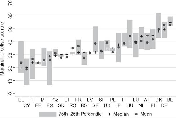
Figure 24.1 Marginal effective tax rates across the EU, 2007 (%). Notes: Countries are ranked by median METR. Source: Jara and Tumino (2013), using EUROMOD.
Union.[531] The scope of these calculations is usually limited to direct taxes and (cash) benefits and current work incentives, though extensions also account for consumption taxes and taking a life-cycle labor supply perspective (see Kotlikoff and Rapson, 2007). Graphically, METRs can be illustrated with a budget constraint chart that plots net income against gross earnings (or hours worked) (see Adam et al., 2006b; Morawski and Myck, 2010), as the slope of this line corresponds to 1 — METR which is the proportion of additional gross earnings retained by the individual.
Participation tax rates (PTR) are conceptually very similar, indicating the effective tax rate on the extensive margin, or the proportion of earnings paid as taxes and lost due to benefit withdrawal if a person moves from inactivity or unemployment to work. METRs and PTRs are typically between 0% and 100%, with higher rates implying weaker incentives to work (more). Because of nonlinearities and complex interactions in the taxbenefit systems, however, individuals facing greater than 100% (or negative) tax rates may also be found. These often expose unintended effects built into the tax-benefit system. More generally, relatively high values indicate situations that can constrain labor supply and trap people at certain income/employment levels. Marginal effective tax rates and participation tax rates are hence useful indicators to assess whether the tax-benefit system may limit employment for certain individuals. These are also central parameters in assessing optimal tax design. See Immervoll et al. (2007) and Brewer et al. (2010) for empirical applications. Figure 24.1 illustrates how in many countries there is a considerable spread in the value of the METRs even before considering the extremes of the distributions. This demonstrates how an analysis using work incentive indicators based on calculations for average or representative cases may be quite misleading.
Replacement rates (RR) complement participation tax rates, showing the level of out- of-work income relative to in-work disposable income (see, e.g., Immervoll and O’Donoghue, 2004). High replacement rates also reflect low financial incentives to become (or remain) employed. Compared to METRs and PTRs, negative values are even more exceptional (though not ruled out altogether). RRs are often calculated separately for the short-term and long-term unemployed to reflect differences in the level of unemployment benefits depending on unemployment duration. As work incentive indicators, PTRs and RRs are calculated for nonworking persons for whom potential employment income is not observed, and, hence, the latter must be either predicted or assumed.[532]
Although PTRs and RRs both describe work incentives on the extensive margin, they have a different focus and characteristics (Adam et al., 2006a). For instance, if taxes and benefits are changed so that net income increases by the same amount for the out-ofwork and in-work situation (e.g., corresponding to a lump-sum transfer), then the replacement rate would typically increase while the participation rate remained unchanged. This is because the tax burden on additional income does not change while, in relative terms, working becomes less attractive. On the other hand, RRs remain constant if out-of-work and in-work net income increase by the same proportion (but for PTRs this is not the case).
Although these three indicators are used to measure work incentives for a particular individual by changing individual gross earnings (and labor market status), the effect on disposable income is assessed at the household level because this is usually considered to be the more relevant unit of assessment for benefits and unit of aggregation when measuring living standards.[533] Each measure can be also decomposed to show the effect of specific tax-benefit instruments, for example, income taxes, social insurance contributions, and benefits.
24.2.2.2 Indicators of Automatic Stabilization
Another closely related group of indicators characterize how tax-benefit systems act as automatic stabilizers for income or unemployment shocks, as indicated by the extent to which (aggregate) household income or tax revenue fluctuations are moderated without direct government action. These focus on exogenous shocks rather than individual incentives to alter labor supply. Apart from this, the calculations are technically very similar to the previous group, with the main differences related to interpretation.[534]
Estimates based on microdata go back at least to Pechman (1973), who simulated income tax revenues in the US for 1954—1971 and showed how much tax liabilities change in absolute terms compared to changes in income (at the aggregate level), characterized as built-in flexibility. Although this is very similar to marginal effective tax rates, the interpretation is different and focused on the macro-level and government revenue side rather than at the individual. A closely related measure captures the elasticity of tax liability with respect to changes in incomes, or percentage increase in taxes for a 1% change in income, though as Auerbach and Feenberg (2000) point out, this mainly reflects the progressivity of taxes because it does not capture whether the tax burden is high or low.
More recently, Auerbach and Feenberg (2000) estimate the aggregate change in taxes when increasing all (taxable) income (and deductions) for each individual by 1% to measure the responsiveness of tax revenues to income changes for the US. They find that, over the period 1962—1995, income taxes offset between 18% and 28% of variation in before-tax income (at the aggregate level). Similarly, Mabbett and Schelke (2007) simulate a 10% increase in individual earnings for 14 EU countries and estimate both the responsiveness (i.e., elasticity) of various tax-benefit instruments and the overall stabilization effect of the system. According to their estimates, the latter varies from 31% in Spain to 57% in Denmark.
Dolls et al. (2012) model a negative income shock in which household gross incomes fall by 5% and an unemployment shock with household income at the aggregate level decreasing also by 5%, covering both the US and a large number of the EU countries. Although the proportional income shock is distribution-neutral, the unemployment shock is asymmetric because not all households are affected. They find that tax-benefit systems absorb a greater proportion ofincome variation in the EU compared to the US— 38% (EU) versus 32% (US) of the income shock and 47% (EU) versus 34% (US) of the unemployment shock (see Figure 24.2). This difference is largely explained by the higher coverage and generosity of unemployment benefits in Europe. Automatic stabilizers in the case of an unemployment shock are basically replacement rates for a transition from employment to nonwork at the aggregate level. Rather than work incentives (as discussed in the previous section), they reflect how much the tax-benefit system absorbs (market) income losses due to becoming unemployed or exiting the labor market altogether.
Instead of focusing on aggregate stabilization, Fernandez Salgado et al. (2014) analyze the distribution of replacement rates when simulating the unemployment shock in six EU
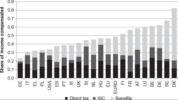
Figure 24.2 Share of income compensated by the tax benefit system in the case of an unemployment shock. Notes: The unemployment shock corresponds to an increase in the unemployment rate such that the total household income decreases by 5%. Countries are ranked by the share of income compensated. EU and EURO are the population-weighted averages of 19 EU and 13 eurozone countries, respectively, included here. Estonia joined the eurozone later and is here excluded from that group. Source: Dolls et al. (2012), using EUROMOD and TAXSIM.
countries due to the Great Recession. They distinguish between short- and long-term unemployment, and their findings confirm higher replacement rates in the short term and point to serious challenges for minimum income schemes to cope with the consequences of this crisis in the longer term. They also highlight the important role of incomes of other household members in boosting replacement rates.
24.2.2.3 Indicators of Household Composition Effects
Another type of indicator based on microsimulation captures the effect of changes in household sociodemographic characteristics in order to identify the marginal effect of the tax-benefit system due to particular household configurations. For example, Figari et al. (2011b) apply this approach to calculate “child contingent” incomes estimated as the change in household disposable income for families with children as if they did not have children. They argue that “child-contingent” incomes, capturing not only transfers net of taxes but also tax concessions, account more precisely for the full net support provided through tax-benefit systems to families with children, as compared to simply considering (gross) benefit payments labeled explicitly for children or families, as is typically the case using the information directly available from the survey data. As shown in Figure 24.3, the net value can be greater than the gross if there are tax concessions or child supplements in benefits labeled for other purposes, and the gross value can be greater than the net if the benefits are taxed or reduced because of other interactions.
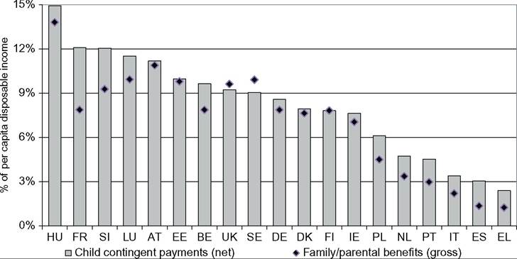
Figure 24.3 Total net child-contingent payments versus gross family/parental benefits per child as a percentage of per capita disposable income. Notes: Countries are ranked by total net child-contingent payments. Source: Figari et al. (2011b), using EUROMOD.
24.3.