THE EFFECTS OF POLICY CHANGES ON INCOME DISTRIBUTION
24.3.1 A Basic Example
The simplest use of a tax-benefit microsimulation model involves calculating the effects of a policy change on household income, without changing any of the characteristics of the household members.
An example might be an increase in the amount of an existing universal child benefit. The model would take account of the increase in payment per eligible child, any clawback through the system of means-tested benefits (if the child benefit is included in the income assessment for these benefits), any clawback if the benefit is taxed or included in the base for contributions, and any other relevant interaction with the rest of the tax-benefit system. Even a simple reform involves quite complicated arithmetic and ignoring the interactions would give misleading results. This is illustrated in Appendix A with a concrete example comparing the effects of doubling the UK child benefit at two points in time: 2001 and 2013. Although the structure of child benefit itself has remained the same, the net effect of changes to it is quite different because of changes to the interactions with the rest of the tax-benefit system. The interactions matter and need to be accounted for in understanding the effects of policy changes and in designing policy reforms.The financing of such a reform would also need to be considered. For example, if the net cost was met by a percentage point increase in all rates of income tax, this increase might also have knock-on effects (e.g., if the assessment of any means-tested benefits depended on after-tax income), and then iterations of the model would be needed to find a revenue-neutral solution to the tax rate increase. The “revenue neutral” package could then be evaluated relative to the prereform situation, in terms of its effect on the income distribution and an analysis of gainers and losers.
Of course, in the new situation some people affected will wish to change their behavior in response to the change in some way and at some point in time. One might expect labor supply and fertility to be affected and, depending on the specifics of the system and the change in it, so might other dimensions of behavior. As Bourguignon and Spadaro (2006) point out, it is important to be clear about when these second order effects can, and cannot, be neglected. We return to this issue in Section 24.3.3.
In any case, an “overnight” or “morning after” analysis, as the pure arithmetic effect is often called, is clearly of value in its own right as the immediate effect might be relevant to a particular research question. Moreover, the mechanics of the way in which policy reforms impact on incomes are relevant for improving design, and it will often be important to identify how much of the overall effect on income can be attributed to the direct effect.
24.3.2 Formal Framework
24.3.2.1 Decomposing Static Policy Effects
Tax-benefit models provide information on the distribution of household disposable income and its components under various policy scenarios, allowing the effects ofpolicies to be inferred from a comparison of different scenarios. As such, the application of the microsimulation method starts by defining an appropriate baseline and a counterfactual scenario. The latter corresponds to the state after policy changes (i.e., how the world would look after implementing new policies) in forward-looking analysis or the state before policy changes (i.e., how the world would have looked without new policies or what would happen if policy changes where rolled back) in the case of backward-looking analysis.
Drawing on Bargain and Callan (2010) and Bargain (2012a), we provide a formal framework for decomposing changes in household income to separate the effects of policy changes.[535] Mathematical formulation helps to avoid ambiguities about how exactly a counterfactual scenario is defined, which often arise in empirical microsimulation applications relying only on textual descriptions.
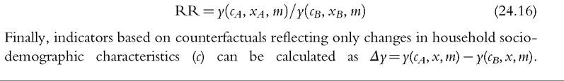
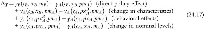
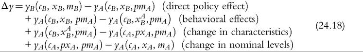
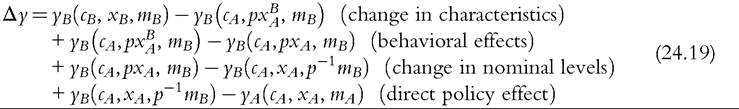
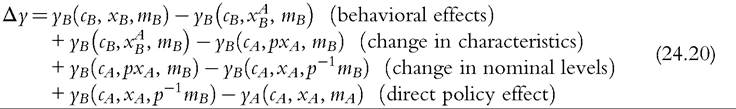
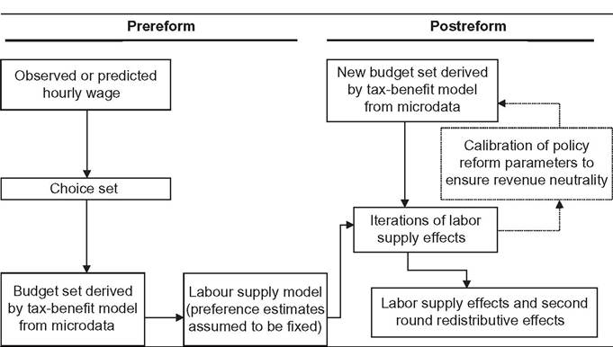
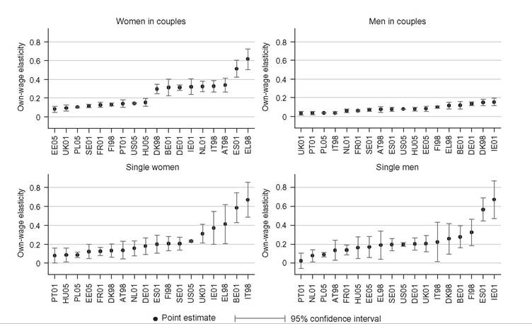
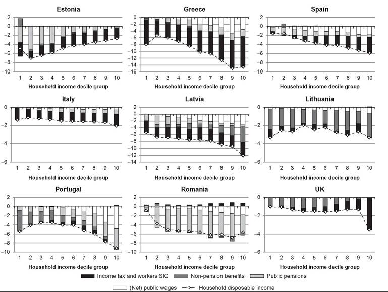
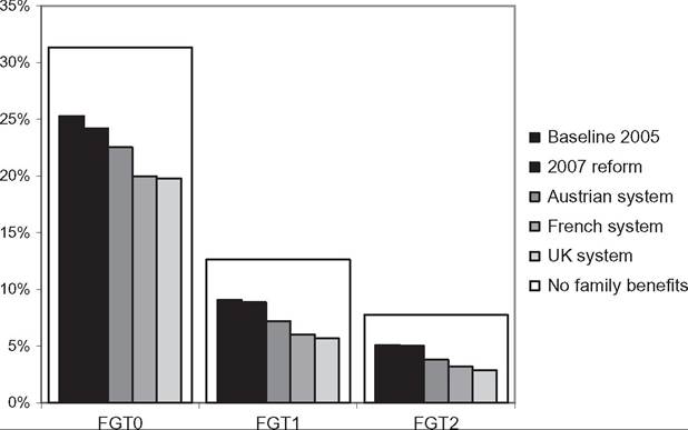
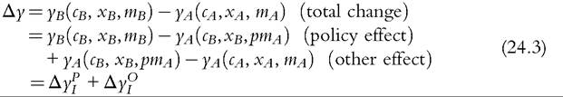
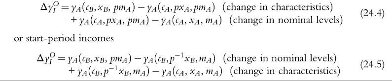
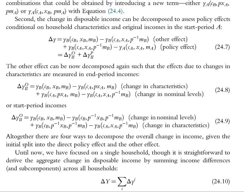
Furthermore, full decomposition (rather than only focusing on the role of policy changes) has clear advantages by drawing attention to the fact that the (marginal) contribution of a given component is evaluated conditional on the values of other components, and, hence, the overall change in income can be decomposed in multiple ways. Decomposing all components (at once) also helps to ensure that these are consistently derived. Apart from small technical modifications,11 we closely follow Bargain and Callan’s original approach but broaden its scope by showing that a wider range of applications can be interpreted within the same framework.Let us denote household sociodemographic (and labor market) characteristics with a vector c and household original income[536] [537] (i.e., income before adding cash benefits and deducting direct taxes) with a vector x. The net transfer via the tax-benefit system k (i.e., total cash benefit entitlement less total direct tax liability) for a household with characteristics c and income x is denoted as a function fk(c, x, mk), where, following Bargain and Callan (2010), we distinguish between the structure of the tax-benefit system fk and the various monetary parameters mk it takes as arguments (e.g., tax brackets, benefit amounts). fk(c, x, mk) is positive if public pensions and cash benefits received by a given household exceed direct taxes for which the household is liable, and it is negative if the opposite holds. Household disposable income y is then In the simplest case, where original income and household characteristics can be assumed to remain constant, the effect of policy changes (A → B) on disposable income is This corresponds to how the effects of proposed or hypothetical tax-benefit reforms are typically studied, as “morning-after” changes with the policy rules before and after referring (implicitly) to the same time period. Next, let us consider the case of analyzing the effect of policy changes over time. Accounting explicitly for the time span over which policy changes are considered introduces additional complexities for defining an alternative scenario. It is important to ensure that the baseline and the counterfactual refer to the same time period, and if there is a time gap between the existing policies and the counterfactual, then one or the other must be adjusted to reflect that. For example, when analyzing the effect of policy change in t + 1, it may not be sufficient to assume that the alternative would have been simply period t policies continuing (in nominal terms) in period t + 1, even though this is often implicitly done. One should consider how existing policies in nominal terms would have evolved otherwise, given the legal rules or usual practice of indexation of policy parameters, or should have evolved. The importance of the time factor becomes even more obvious when considering policy changes over a longer period. We will return later to the question of what is an appropriate basis for indexing monetary parameters in the counterfactual scenario, but for now we simply denote such a factor as p. First, the total change in disposable income for a given household can be decomposed to show first order policy effects (or mechanical effects) conditional on household characteristics and original incomes in the end-period B (denoting the start-period with A): Here we are implicitly assuming that we are dealing with panel data, with characteristics and original income for the same household being observed in several periods. The total change for the same household cannot be observed with multiple waves of cross-sectional datasets; however, as explained further below, the same decomposition approach can be also applied at the group-level (e.g., the bottom decile group) or to statistics summarizing the whole income distribution (such as various inequality indices). Noting the symmetry of the decomposition, the other effect can be decomposed further into two subcomponents separating the impact of change in household characteristics and nominal levels. The effect due to changes in characteristics can be measured either in end-period income levels: The term capturing the effect of “change in nominal levels” measures how household disposable income is affected if original income and all money-metric policy parameters change in the same proportion. As Bargain and Callan (2010) pointed out, tax-benefit systems are typically homogenous of degree 1, meaning that in such a case, household disposable income would also change by the same factor: They illustrate this with a hypothetical example involving a basic income and a flat tax and find empirical support for Ireland and France.[538] In principle, the term reflecting the impact of changes in characteristics could be split further, distinguishing between changes in sociodemographic (and labor market) characteristics c and movements in original incomes x. Again, there would be two possible In the case of scale-invariant distributional measures (see Cowell, 2000) and linearly homogenous tax-benefit systems, the decomposition of other effects (Equations 24.4, 24.5, 24.8, 24.9) simplifies because the effect of a change in nominal levels becomes (approximately) zero at the population level.[539] Furthermore, Equation (24.4) is now equivalent to Equation (24.5), and Equation (24.8) is equivalent to Equation (24.9), reducing the overall number of combinations from four to two. We now return to what would be an appropriate basis for choosing the indexation factor p. Bargain and Callan (2010) have argued for using the growth of average original incomes, expressed as p = xb∕xa, to obtain a “distributionally neutral” benchmark. This would broadly ensure that aggregate disposable income rises (or falls) in proportion to an increase (or a decrease) in aggregate original incomes; in other words, the overall tax burden and expenditure level remain constant in relative terms.[540] Nevertheless, disposable income for a given household could still grow at a higher (or lower) rate than their original income if the latter grows less (or more) than on average. However, there are alternatives ways of choosing p, depending on the chosen conception of “neutrality.” For example, basing it on a consumer price index would be appropriate if the point was to ensure a constant absolute standard of living (on average). Clark and Leicester (2004) contrast price-indexation with indexation based on the nominal GDP, and they show that the choice matters for results. There is no clear consensus in the literature on decomposition regarding the most appropriate choice of index. Finally, there is the issue of how to deal with path dependency and multiple combinations for decomposition. Can some combinations be preferred over others or can different combinations somehow be brought together? In some cases, one might be limited to specific combinations by data constraints. The prime example here is ex ante analysis of (implemented) policy changes before microdata of actual postreform incomes become available (e.g., Avram et al., 2013). Relying on estimates forp, one could already quantify the effect of policy changes (with Equation 24.7), but both start- and end-year datasets are needed to assess other effects. Given that there are no clear arguments for preferring one particular combination over another, all variants should be covered. Bargain and Callan (2010) adopt the Shorrocks-Shapley approach (Shorrocks, 2013) to summarize various combinations, essentially averaging the effect of a given component across all combinations. In this way, results conditional on household characteristics in each period are given equal weights. Other examples where such decomposition has been used explicitly include Bargain (2012b), Bargain et al. (2013b), and Creedy and Herault (2011). In addition, there is a large literature that documents similar assessments within less formal frameworks (for example, see Clark and Leicester, 2004; Thoresen, 2004). 24.3.2.2 Specific Applications 24.3.2.2.1 Actual Versus Counterfactual Indexation of Policy Parameters Any system which is not fully indexed with respect to growth in (average) private incomes or prices would result in the erosion of the relative value of benefit payments and increased tax burden through so-called bracket creep (or fiscal drag). Furthermore, it is essential to acknowledge that keeping a tax-benefit system unchanged also impacts household incomes (unless the distribution of household original income is also constant over time). Let us consider the change in household disposable income in such a case using our notation from above: Following the decomposition framework in the more general case above, Equation (24.12) can be split again into three terms: the policy effect, changes in original incomes, and the change in nominal levels (i.e., change in disposable income ifboth original incomes and policy parameters were scaled up by the same factor). The policy effect 24.3.2.2.2 Policy Swaps An analogous type of exercise to that comparing the effects of policies across time in one country involves assessing the effects of policies from one country (A) when simulated in another (B), the so-called policy swaps. The starting point is again Equation (24.3), but instead of comparing the effects of two different national policy regimes on the same population and distribution of original incomes, the aim is to compare the effects of a particular set of “borrowed” policies on different populations and income distributions. Some studies focus on the effects of several alternative systems in one particular country (one-way swaps), and others carry out two-way swaps sometimes involving more than two countries in a series of swaps. Section 24.3.6 discusses some examples of such studies. Instead of growth in income over time and the relative movement in tax-and benefit parameters, the nature ofp has to do with difference in nominal levels of original income across countries. Often there are additional complexities involved in maintaining correspondence with original policies, especially if more than one pair-wise comparison is made. Attempts so far have aimed to keep the values of parameters fixed in relative terms, for example, in connection to average income or in order to maintain budget neutrality. 24.3.2.2.3 Microsimulation-Based Indicators The same framework can be used to describe microsimulation-based indicators, designed to capture some inherent characteristics of a given tax-benefit system, which are not directly observable. The nature of these was already explained in Section 24.2.2, and here we formalize the key definitions. Overall, these indicators show how household disposable income reacts to changes in people’s gross earnings and circumstances (for a given tax-benefit system): Using our notation, we can express marginal effective tax rates (METR) as follows: where the change in household disposable income is divided by the margin (d) used to increment gross earnings (x) of a given household member, yielding a relative measure. This is further deducted from one to show the part of additional earnings which is taxed away. In the case of participation tax rates (PTR), both earnings (x) and other household characteristics (c) are adjusted to reflect the change in labor market status, as with the change from inactivity or unemployment (A) to work (B): The relative income change is again deducted from one to reflect the effective tax rate at this margin. (Note that this could be further simplified as xA = 0.) Replacement rates (RR) are simply calculated as the ratio of out-of-work disposable income (A) to in-work disposable income (B): For example, “child-contingent” incomes would show the change in household disposable income for families with children (A) compared to the income if they did not have children (B). 24.3.2.3 Decomposition With Labor Supply Changes So far we have focused on the static effects of policy changes, whereby potential behavioral reactions have been absorbed by the component capturing changes in household characteristics more generally. Following Bargain (2012a), we now extend the previous case and explicitly account for behavioral changes in the form of labor supply adjustments due to policy changes. For this purpose, we slightly change the notation from xk to xlk, which refers to original incomes by population with characteristics ⅛ based on labor supply choices made under the policy system l. (As such, the meaning of x⅛ is exactly the same as xk before and, hence, will be shortened to the latter.) This allows the term “changes in characteristics” to be further split into two components—labor supply adjustments following changes in policy rules (A → B) and other effects due to changes in the population structure c (assumed to be exogenous to tax-benefit policy changes, at least in the short and the medium term). We can now express the overall change in household disposable income as a sum of four components: direct (or mechanical) policy effect, labor supply reactions, change in nominal levels, and change in characteristics. Decomposing Equation (24.4) and combining it with Equation (24.3), we can separate the behavioral effects comparing disposable income with labor supply under the initial and the new policy rules, expressed in terms of initial policy rules (yA, pmA) and either start-period household characteristics cA: or end-period household characteristics cB Decomposing Equation (24.8) instead and combining it with Equation (24.7) allow the behavioral effects to be expressed in terms of new policy rules (yB, mB) and, again, start-period household characteristics cA: or end-period household characteristics cB[541]: Modeling behavior and in particular labor supply is discussed in more detail in the next section. 24.3.3 Modeling Behavioral Changes 24.3.3.1 Accounting for Individual Reactions The impact of policies on individual behavior, through incentives and constraints, is at the core of economics, and behavioral microsimulation models are valuable tools for providing insights into the potential behavioral reactions to changes in the tax-benefit system and, consequently, on their effect on economic efficiency, income distribution, and individual welfare (Creedy and Duncan, 2002). Nevertheless, it is important to be clear when the second-order effects can, and cannot, be neglected. To capture the individual effect of reforms, it is not always necessary to quantify behavioral responses, on the assumption that the effects of the policy changes are marginal to the budget constraint (Bourguignon and Spadaro, 2006). Of course, it is not possible to judge a priori whether the behavioral response is large or ignorable. Judgments must necessarily be made on an ad hoc basis, using available evidence and related to the context of the analysis and how results are to be interpreted. If behavior is known to be constrained (e.g., in the case oflabor supply adjustments at times of high unemployment), then behavioral responses might be ignored, and it is sufficient to consider the results of the analysis in terms of changes in income (rather than welfare). If static indicators of work incentives, such as marginal effective tax rates and participation tax rates, change very little as a result of a policy change, then one can assume that labor supply responses driven by substitution effects will be small. If the change in income with and without modeled behavioral response is expected to be rather similar, then given the error in the modeling of behavior and in the static microsimulation estimates themselves, going to the trouble of modeling responses may not be worthwhile (Pudney and Sutherland, 1996). Moreover, being clear about the relevant time period is important. From a policymaking viewpoint, it is the effect on the income distribution and on the public budget in the year of the reform that often matters. Most tax and benefit policy changes are made year to year and are fine-tuned later if necessary. On the one hand, behavior takes time to adapt to changing policies, partly because of constraints, adjustment costs, and lack of information or understanding. This applies most obviously to fertility but also to labor supply in systems where full information about the policy rules is not available until the end of the year (after labor supply decisions have already been acted on). On the other hand, changes in behavior may also happen in anticipation of the policy being implemented, with short-term responses larger than long-terms effects. This may apply particularly to tax planning behavior and is well-illustrated by the case of an announcement in the UK in 2009 of a large increase in the top rate of tax on high incomes in the 2010—2011 tax year. Major forestalling of income by those who would pay the additional tax and were in a position to manipulate the timing of their income resulted in an unexpected increase in tax revenue in the 2009—2010 tax year and a corresponding reduction in the following year (HMRC, 2012). In some situations the morning-after effect is the most relevant when considering short-term policy adjustments and equilibrium (or partial equilibrium) considerations are not particularly relevant. Furthermore, if indicative results are needed quickly because reform is imperative, then in the absence of an already-estimated and tested behavioral model, static results with the appropriate “health warnings” are still more informative than nothing at all. Nevertheless, it is widely recognized that, depending on the policy change being analyzed, ignoring behavioral reactions can lead to misleading estimates of the impact of the policy reform on the income distribution and the macroeconomic consequences (Bourguignon and Spadaro, 2006), as is also illustrated by the tax-planning example. At the other extreme, modeling behavioral responses in the case of very large changes to policy poses challenges for the empirical basis of behavioral modeling. For example, replacing an existing tax-benefit system with a combination of a basic income and a flat tax such that no income fell below the poverty threshold would presumably result in large changes in many dimensions of behavior which are unlikely to be correctly captured by the labor supply models that are used traditionally. Despite the long tradition of modeling behavior in economics, the behavioral reactions to changes in the tax system that are most commonly analyzed are related to labor supply (starting with the seminal contributions of Aaberge et al., 1995 and van Soest, 1995) and program participation (Keane and Moffitt, 1998), feeding into a growing literature, which is characterized by an increasing level of econometric sophistication. The same level of development does not yet apply to other research areas in which microsimulation models have been used, such as investigating the potential effects of tax policies on consumption (Creedy, 1999b; Decoster et al., 2010), saving (Boadway and Wildasin, 1995; Feldstein and Feenberg, 1983), and housing (King, 1983), at least partly due to a lack of suitable data. 24.3.3.2 Labor Supply Models There is a general consensus in the literature about using (static) discrete choice models to simulate the individual labor supply reactions to changes in the tax-benefit system.[542] Such models are structural because they provide direct estimations of preferences over income and hours of work, through the specification of the functional form of the utility function. Discrete choice models belong to the family of random utility maximization models (McFadden, 1974) that allow the utility function to have a random component (usually following the extreme value distribution), affecting the optimal alternative in terms of utility level associated with each choice. The discrete choice character of the models is due to the assumption that utilitymaximizing individuals and couples choose from a relatively small number of working hour combinations, which form the personal choice set. Each point in the choice set corresponds to a certain level of disposable income given the gross earnings of each individual (derived using the observed or predicted wage), other incomes, and the tax-benefit system rules simulated by means of a tax-benefit microsimulation model taking into account the sociodemographic characteristics of the family. The nonlinear and noncon- vex budget sets determined by complex tax-benefit systems provide a primary source of identification of the model itself. Most of the discrete choice models based on the van Soest (1995) approach assume that the same choice sets are defined and available for each individual and that an individual has the same gross hourly wage for each such alternative. Ilmakunnas and Pudney (1990) is one of the few exceptions in the literature, allowing the hourly wage to be different according to the number of hours offered by each individual. Aaberge et al. (1995) provide a more flexible specification that defines the alternatives faced by the individuals in terms of a set of a wage rate, hours of work, and other job-related characteristics. The wage rate can differ for the same individual across alternatives, the hours of work are sampled from the observed distribution, and the availability of jobs of different types can depend on individual and institutional characteristics. Regardless of the econometric specifications, the sample is usually restricted to individuals who are considered “labor supply-flexible” in order to exclude individuals whose labor choices are affected by factors that are not or cannot be controlled for in the labor supply model. Examples of these factors include disability status, educational choices, early retirement, and self-employment status. This represents a limit in the use of the estimated labor supply responses to analyze changes in overall income distribution because, for the individuals not covered by the labor supply models, the behavior is assumed to be inelastic. In most applications, working age individuals within the family are allowed to vary their labor supply independently of each other, and the utility maximization takes place at the family level, considering the income of both partners subject to a pooled income constraint, in line with the unitary model of household behavior. Blundell et al. (2007) provides an example of the structural model of labor supply in a collective setting, excluding the effects of taxes. 17 Figure 24.4 depicts the main components of a standard labor supply model that uses a static tax-benefit algorithm to generate input for the labor supply estimation and to evaluate the labor supply reactions to policy reforms. In the prereform scenario (left panel of Figure 24.4), the labor supply model is estimated on the budget set providing a direct estimate of the preferences over income and hours. In the postreform scenario (right panel of Figure 24.4), a new budget set for each family is derived by the tax-benefit model applying the new tax-benefit rules following the simulated reform. Assuming that individual random preference heterogeneity and observable preferences do not vary over time, labor supply estimates from the prereform scenario are used to predict the labor supply effects and the second-round redistributive effects (i.e., when labor supply reactions are taken into account) of the simulated policy reforms. Such effects might come out of an iterative procedure calibrating the policy parameters to ensure revenue neutrality once the labor supply reactions and their effects on tax revenue and benefit expenditure are taken into account. Figure 24.4 Behavioral tax-benefit model and underlying data. Applications of discrete choice behavioral models are too numerous to be surveyed in this context. Alongwith many applications focused on the potential effects of specific taxbenefit policies (among others, see Brewer et al. (2009) for a review of analysis of the effects of in-work benefits across countries), labor supply models based on microsimulation models provide labor supply elasticities that can be used in other tax policy research (e.g., Immervoll et al., 2007). Using EUROMOD and TAXSIM, Bargain et al. (2014) provide the first large-scale international comparison of labor supply elasticities including 17 EU countries and the US. The use of a harmonized approach provides results that are more robust to possible measurement differences that would otherwise arise from the use of different data, microsimulation models and methodological choices. Figure 24.5 shows the estimated own-wage elasticities for single individuals and individuals in couples, which suggest substantial scope for the potential impact of tax-benefit reforms on labor supply and hence income distribution, though the differences across countries are found to be smaller with respect to those in previous studies. Bargain et al. (2014) also show the extent to which labor supply elasticities vary with income level which has important implications for the analysis of the equity-efficiency trade off inherent in tax-benefit reforms. To this aim, labor supply models can be used to implement a computational approach to the optimal taxation problem, allowing the empirical identification of the optimal income tax rules according to various social welfare criteria under the constraint of revenue neutrality (Aaberge and Colombino, 2013). Figure 24.5 Europe and United States: Own-wage elasticities. Source: Bargain et al. (2014), using EUROMOD and TAXSIM. The rapid dissemination of labor supply models, no longer restricted to the academic sphere and increasingly used to inform the policy debate, has been accompanied by a continuing refinement of the econometric specifications. Nevertheless, further improvements are still necessary to model the labor market equilibrium that can emerge as a consequence of a policy simulation (Colombino, 2013), to take into account demand side constraints (Peichl and Siegloch, 2012) and to exploit the longitudinal dimension of micro-data, where this is available, in order to avoid labor supply estimates being potentially biased by individual unobserved characteristics and to consider the state dependence in the labor supply behavior (Haan, 2010). 24.3.3 Macroeconomic Effects In a basic application of a static microsimulation model, labor market conditions and levels of market income are taken from the underlying data without further adjustments. However, these conditions may change due to policy, and economic and institutional changes, and in order to assess the social consequences of macroeconomic changes, it is important to consider the interactions of the tax-benefit system with new conditions in the labor market and with other macroeconomic effects in general. On the one hand, micro-oriented policies can have a second round effect due to micro-macro feedbacks: for example, a generous income support scheme can have effects on labor market and saving behaviors. On the other hand, macro-oriented policies or exogenous shocks have a redistributive impact that needs to be assessed if the potential implications for the political economy of the reforms is to be understood (Bourguignon and Bussolo, 2013). As in the case of a policy change, the microsimulation approach can offer insights in two ways. First, it can provide, in a timely fashion, an ex-ante assessment of how individuals are affected by the macroeconomic changes, either actual or hypothetical. Second, it can be used to develop a counterfactual scenario to disentangle ex-post what would have happened without a given component of the macroeconomic shock. However, in order to capture the consequences of a macroeconomic shock on income distribution, a partial equilibrium setting at the micro level can be too limited. Thus, it is necessary to capture the interactions of the tax-benefit system with population heterogeneity observed at the micro level, as well as the macro changes in the fundamentals of an economy due to policy reforms or exogenous shocks.[543] In the last decade, the growing literature has explored different ways to link micro and macro models (often belonging to the family of computational general equilibrium (CGE) models), yet the construction of a comprehensive, policy-oriented micro-macro economic model still faces many challenging issues. Although it is now quite common to see disaggregated information from micro-level data used in a macro model (i.e., using the parameters of behavioral models or the effective tax rates simulated by microsimulation models in CGE models), it is rarer to see a fully developed microsimulation model being integrated with a macro model. See Bourguignon and Bussolo (2013) for an excellent review of the different approaches. The simplest and widely implemented way to combine micro and macro models is the top-down approach. Robilliard et al. (2008) provide an example of sequentially combining a microsimulation model with a standard multisector CGE model, not only focusing on the labor markets but also on the expenditure side taking into account the heterogeneity of consumption behavior of individuals. First, the macro model predicts the linkage variables, such as new vectors of prices, wages, and aggregate employment variables that are the consequences of a macroeconomic shock or a new policy. Second, the microsimulation model generates new individual earnings and employment status variables consistent with the aggregates from the macro model and hence simulates a new income distribution. In such a top-down approach, the potential macro feedback effects of the new situation faced by the individual are not taken into account specifically, but only through the representative households embedded in the macro model. Because it depends on the aggregation of behavior at the individual level, this approach can only provide the first-round effects of the exogenous (policy) change. Bourguignon et al. (2005) extend the top-down approach by including in the microsimulation model the behavioral reactions of individuals to the price changes predicted by the macro model. In contrast, in the bottom-up approach, the individual behavioral changes due to a policy reform are simulated at the micro level and then aggregated to feed into the macro model as an exogenous variation in order to analyze the overall effect on the economy. Any feedback effect from the macro model back into the microeconomic behavior is ignored in this setting (Brown et al., 2009). A more complete recursive approach is given by the combination of the two approaches through a series of iterations until effectively no further adjustments are observed, in order to take into account the feedbacks that would otherwise be ignored and to arrive at a fully integrated macro-micro model. In the macro part of such a model, the household sector is not given by a few representative households but by the microlevel sample of households representative of the whole population. Aaberge et al. (2007) is an example of the integration between a labor supply microsimulation model and a CGE model in order to assess the fiscal sustainability of the aging population in Norway. Peichl (2009) uses the same approach to evaluate a flat tax reform in Germany. Considering the efforts needed to develop a fully integrated model, the choice of the appropriate approach depends on the research or policy question at hand, and more parsimonious models can do the job in many circumstances. Notwithstanding, a fully integrated micro-macro model, as suggested by Orcutt et al. (1976), would be an incredibly powerful tool for building counterfactuals taking into account feedback effects between the micro and macro levels and for disentangling the effect of a given macro change on individual resources and hence on income distribution. 24.3.5 Predicting Income Distribution Using microsimulation to predict income distribution is an area of work that is fueled by the need of policymakers to have more up-to-date estimates of poverty and inequality and the effects of policy than can be supplied directly from micro-data that are usually 2-3 years out of date. This need is particularly acute if indicators ofincome distribution are to be taken into account in assessments of economic and social conditions alongside aggregate economic indicators, which are generally available in a more timely way (Atkinson and Marlier, 2010; Stiglitz, 2012). Furthermore, the practice of setting targets for the future achievement of social goals is becoming more widespread. In relation to poverty and income distribution, this applies particularly in the European Union through the Europe 2020 targets for the risk ofpoverty and social exclusion,[544] and in the developing world through the UN Millennium Development Goal for the eradication of hunger and extreme poverty.[545] Predictions ofthe current situation, known as “nowcasts,” are valuable indicators for measuring the direction and extent of movement toward the associated targets, along with predictions for the target date at some future point (i.e., forecasts). The approaches for predicting income distribution also depend on the time framework of the analysis. Methods for nowcasting and forecasting are distinct in the sense that the latter must rely on assumptions or other forecasts about the economic and demographic situation, as well as the evolution of policies, rather than recent indicators, data, and known policy parameters. However, the choice of techniques is common to both, and before discussing the two time frameworks in turn, the next subsection considers a key issue: how to model changes in labor market status. 24.3.5.1 Modeling Changes in Labor Market Status In order to capture the effects of exogenous changes in economic status on income distribution, two techniques can be implemented at the micro level. One approach is to reweight the data (Creedy, 2004; Gomulka, 1992; Merz, 1986), and another approach is to model transitions from one status to another at the individual level (Fernandez Salgado et al., 2014). Reweighting is commonly used because it is relatively straightforward to carry out and to test the effects of alternative specifications. For example, to model an increase in the unemployment rate (Immervoll et al., 2006b), the survey weights of households containing unemployed people at the time of the survey must be increased, and the weights of other similar households reduced, in order to keep demographic characteristics and household structures constant in other relevant dimensions. Following this approach, Dolls et al. (2012) simulate a hypothetical unemployment shock in 19 European countries and the US in order to analyze the effectiveness of the tax and transfer systems to act as an automatic stabilizer in an economic crisis. However, the main disadvantage of the reweighting approach, especially in the context of a rapidly changing labor market, is that it assigns the characteristics of the “old” unemployed (in the original data) to the “new” unemployed (corresponding to the current period). To the extent that the unemployed in the data were long-term unemployed, this will underestimate the number of new unemployed in receipt of unemployment insurance benefits, which are time-limited in most countries, and overestimate the extent to which incomes are lowered by unemployment. Furthermore, the unemployment shock may have affected certain industries and occupations more than others. Another drawback of reweighting is that it can result in very high weights for some observations, which can distort the results of simulations affecting dimensions not controlled for. In addition, although the implications of alternative formulations for the empirical results are straightforward to explore, it is far less straightforward to assess the statistical properties and reliability of the weights themselves, given that for any one set of weights satisfying the calibration constraints, there are also others (Gomulka, 1992). Moreover, reweighting does not permit the modeller to account for the interactions between changes in the individual status and different tax-benefit instruments, for example, to analyze to what extent the welfare system counterbalances income losses specifically for those who became unemployed, rather than at the aggregate level. This is possible with the second approach, which involves explicit modeling of transitions at the individual level, making use of external information about the changes occurring in a given dimension. In principle, the full range of relevant characteristics of the people affected can be taken into account. An explicit simulation allows for the detailed effects of tax and benefit policy to be captured for those making the transition. In other words, it allows the production of quasi “panel data” that tracks the same individual before and after a given change, disentangling what would have happened without the change and highlighting the interactions of the tax-benefit system with the individual sociodemographic characteristics. Following this approach, Fernandez Salgado et al. (2014) simulate individual transitions from employment to unemployment at the onset of the Great Recession in six European countries. As a consequence of the macroeconomic shock, household incomes of individuals who lose their jobs are predicted, considering the direct cushioning effect of the tax-benefit systems and the way they depend on the market income of other household members and personal/household characteristics. The comparison between incomes before and after the shock provides a way to stress-test the tax-benefit systems, assessing the relative and absolute welfare state resilience. To date there have been few systematic comparisons of reweighting versus the explicit simulation of individual transitions. Herault (2010) provides a comparison of results using the two methods on South African data and concludes that “the reweighting approach can constitute a good alternative when data or time constraints do not allow the use of the behavioral approach and when the production of individual level transition matrices in and out of employment is not essential” (p. 41). 24.3.5.2 Nowcasting Tax-benefit microsimulation models have for many years been used to simulate the effects of the most recent policies so that ex ante analysis of policy reforms can take the current situation as the starting point. In doing this, it is necessary to update the input micro-data to reflect current economic and social conditions. This might be done with varying degrees of sophistication depending on the question at hand and the amount of change in relevant dimensions between the reference period of the micro-data and the reference year of the policy. Usually, information in the data on original income is updated using appropriate indexes. In addition, the sample might be reweighted to account for certain demographic and economic changes (see section 24.3.5.1). The simulated distribution of household disposable income, based on adjusted population characteristics, updated original income, and simulated taxes and benefits using current rules, is then assumed to be a reasonable representation of the current income distribution.2 However, in times of rapid change, two factors suggest that this approach may not be adequate. First, simple reweighting cannot generally capture major changes accurately, and income growth may vary greatly around the mean, requiring a disaggregated approach. Most obviously this applies in the case of an economic downturn and a sudden increase in unemployment with its asymmetric effects, or an upturn and an increase in employment, when, as is typically the case, the impact is uneven across the population. Secondly, it is at times of rapid change or economic crisis that policymakers particularly need to know about very recent movements in the income distribution and the current situation rather than those a few years previously. The same applies in times of growth if policymakers are concerned about some sections of the population being left behind. Furthermore, in times of crisis, fiscal stimulus or fiscal consolidation policies may play a particularly important role in reshaping income distribution. A microsimulation approach has particular advantages because it captures the specific impact of the components of these policy packages that have a direct effect on household incomes, as well as their interactions with changing market incomes. In times of rapid growth, fiscal drag will typically have distributional consequences (see Section 24.3.2.2), which will be important for policymakers to anticipate if they wish to prevent relative poverty from rising (Sutherland et al., 2008). 21 See for example Redmond et al. (1998) and Callan et al. (1999). Borrowing the term nowcasting from macroeconomics (see, for example, Banbura et al., 2011) the use of an extended and refined set of microsimulation methods in combination with timely macroeconomic statistics is able to provide estimates of the current income distribution using micro-data on household income which are typically 2 or more years out of date. These methods include: (a) updating market incomes from the income data year to current (or latest), using published indexes with as much disaggregation as these statistics allow and from the latest to “now” according to macro-level forecasts or assumptions; (b) simulating policy changes between the income data year to those prevailing currently; (c) adjusting data to account for important dimensions of actual labor market change between the data year and the most recently available information; (d) adjusting data to account for actual and projected demographic and other compositional changes (e.g., household composition) between the data year and “now.”[546] [547] An early attempt to use these methods to update poverty statistics for the UK is pro- videdby de Vos and Zaidi (1996). More recently, these methods have been used to nowcast the policy effects of the crisis in Ireland (Keane et al., 2013); to examine the distributional effects of the crisis in Greece (Matsaganis and Leventi, 2013); and to nowcast the income distribution in Ireland (Nolan et al., 2013), the UK (Brewer et al., 2013), and Italy (Brandolini et al., 2013). They have also been used for eight European Union countries to nowcast the risk of poverty, using EUROMOD (Navicke et al., 2014). A key issue for all the studies that aim to nowcast income distribution in (or on the way out of) the Great Recession, using prerecession data, is to capture labor market changes with sufficient precision. The same would apply during a period of increasing employment rates. Most of the studies cited above use reweighting to adjust for both demographic and labor market changes. The study by Navicke et al. (2014) is an exception. Holding demographic factors constant, it used explicit simulation of labor market transitions to capture the very specific and varied incidence of unemployment across the eight countries considered in the relevant period. The method is based on that employed by Figari et al. (2011c), using Labor Force Survey (LFS) statistics to establish the required number of transitions of each type according to personal characteristics. The microsimulation model, in this case EUROMOD, then selects from the available pool of people with these characteristics in the input database and changes their status accordingly. Incomes are simulated, accounting for the new status, for example, by calculating eligibility and entitlement to unemployment benefits for those making the transition from employment to unemployment. 24.3.5.3 Forecasting Although nowcasts can make use of very recent indicators of economic and labor market conditions and typically project forward by only a few years, allowing slowly changing factors such as demographic composition to stay the same, forecasts project further in time and must rely on assumptions and predictions from other models. In this sense they are usually better seen as drawing out the implications for the income distribution of a particular economic/demographic scenario. For example, Marx et al. (2012) explore the implications of meeting the Europe 2020 targets for employment for indicators of risk of poverty and social exclusion, finding that the composition of any new employment is a key factor. The World Bank (2013) uses a similar approach to exploring the implications of meeting both the education and employment targets for the poverty indicators in the countries of Eastern Europe. In both cases there is no tax-benefit microsimulation, and it is assumed that tax-benefit effects are the same as those in the underlying micro-data. This is justified on the grounds that future policy reforms are difficult to predict. However, this approach neglects any interactions between sociodemographic and labor market characteristics and the tax-benefit system. Microsimulation can take account of these and, even assuming a constant tax-benefit policy structure and a constant relationship between income levels and tax-benefit parameters, would allow the automatic effects of policies on changing market incomes to be captured. Nevertheless, as explained in Section 24.3.2.2, it is important to be aware that assumptions about the indexation of current policies can have a major effect on distributional outcomes (Sutherland et al., 2008). In some situations enough is known about the probable evolution of policies to include the discretionary tax-benefit reform effects in the predictions, as well as the automatic effects driven by changes in the circumstances of households. In the UK not only are policy reforms often announced several years in advance, but also there is detailed information available about indexation assumptions that are built into official public finance forecasts (HM Treasury, 2013; Table A1), as well as regular and detailed growth and inflation forecasts (OBR, 2013; Table 2.1) that can together be used as baseline assumptions for defining policies in the forecast year. Brewer et al. (2011) have forecast child poverty in 2020, using a combination of these types of assumptions, reweighting, and tax-benefit microsimulation. Such an approach not only provides a prediction (in this case that, given the assumptions, the UK will not meet its target for child poverty reduction in 2020) and allows the drivers of the prediction to be identified (through sensitivity analysis), but it also allows a “what would it take?” analysis to suggest what combinations of reforms and other changes would be needed to meet the target. 24.3.6 Cross Country Comparisons Using Microsimulation Cross-country comparisons of the effects of policies naturally add value to what can be said about a single country because the broader perspective helps to provide a sense of scale and proportion. They provide the basis for assessing the robustness of results and generalizing conclusions. In addition, considering several countries within the same analysis provides a kind of “laboratory” in which to analyze the effects of similar policies in different contexts or different policies with common objectives (Sutherland, 2014). Comparisons can take several forms. At their simplest the effects of different policies or policy reforms in different countries can be analyzed side-by side. Bargain and Callan’s (2010) decomposition analysis for France and Ireland is one example of this approach. Another is Avram et al. (2013) who analyze the distributional effects of fiscal consolidation measures within a given period in nine countries. A second approach is to contrast the effects of a common, hypothetical policy reform in several countries, highlighting the relevance of the interactions of a specific policy design with population characteristics and economic conditions. Often the “reform policy” is designed to highlight features of the existing national system that it replaces or supplements. Examples include Atkinson et al. (2002) and Mantovani et al. (2007) for minimum guaranteed pensions, Levy et al. (2007a) for universal child benefits, Callan and Sutherland (1997) for basic income, Bargain and Orsini (2007) and Figari (2010) for in-work benefits, Matsaganis and Flevotomou (2008) for universal housing transfers, Figari et al. (2012b) for the taxation of imputed rent, and Paulus and Peichl (2009) for flat taxes. This type of analysis is usually complicated by the need for the reform policy to be scaled somehow if it is to have an equivalent effect in countries with different levels of income, and because of the need to consider how the reform policies should be integrated with existing national policies. Given that the starting points are different (e.g., the tax systems may treat pensions differently) the net effects will differ, too. A third approach, which was introduced in Section 24.3.2.2, is to swap existing policies across countries in order to explore how their effects differ across different populations and economic circumstances. Examples of this kind of “policy learning” experiment include a comparison of the effectiveness of benefits for the unemployed in Belgium and the Netherlands (De Lathouwer, 1996), as well as many studies of the effectiveness of public support for children and their families: Atkinson et al. (1988) for France and the UK; Levy et al. (2007b) for Austria, Spain and the UK; Levy et al. (2009) for Poland, France, Austria, and the UK; Salanauskaite and Verbist (2013) for Lithuania, Estonia, Hungary, Slovenia, and the Czech Republic; and Popova (2014) who compares Russia with four EU countries. Policy swap analysis can, in principle, be done using a set of national microsimulation models, side by side. But Callan and Sutherland (1997) found that the task of making models produce comparable results was formidable, even forjust two (arguably) relatively similar countries (Ireland and the UK). Thisjustified the construction ofEUROMOD as a multicountry model that now covers all EU member states (see Box 24.1). Indeed, with some exceptions, many of the studies referred to above make use of EUROMOD. As intended, this greatly facilitates cross-country comparability (particularly of the concepts used), the implementation of common reforms using common code and the mechanics of carrying out policy swaps (transferring coded policies from country A to country B). EUROMOD is designed to be as flexible as possible, allowing a huge range of assumptions to be made about cross-country equivalence of different aspects of policy simulation. One example is the treatment of non-take-up of benefits (see Section 24.4.2), and another is the default indexation of policies each year (see Section 24.3.2.2). Thus policy swapping is not a mechanical procedure. Each exercise has its own motivation and corresponding decisions to be made about which aspects of policy (and assumptions driving its impact) are to be “borrowed” from elsewhere and which are to be retained from the existing local situation. Here, we give two empirical examples. The first is an example of side-by-side crosscountry analysis using EUROMOD from Avram et al. (2013). This compares the distributional effects of the fiscal consolidation measures taken in nine European countries in the period up to 2012 from the start of the financial and economic crisis. Figure 24.6 shows the percentage change in average household income due to the measures across the (simulated) 2012 income distribution. The measures include different mixes of increases in income tax and social contributions and cuts in public pensions, other cash benefits, and public sector pay. Four things are striking about this figure and serve to demonstrate the added value of cross-country comparisons of this type, relative to single country studies. First, the scale of the effect varies greatly across the countries (noting that the country charts are drawn to different scales, but the grid interval is uniformly 2% points), ranging from a drop in income on average from 1.6% in Italy to 11.6% in Greece. Second, the choices made by governments about which instruments to use differ across countries. Third, the incidence of the particular changes is not necessarily as one might expect a priori. For example, increases in income tax have a roughly proportional effect in many countries and are concentrated on higher-income households only in Spain and the UK, as might be expected a priori. Cuts in (contributory parental) benefits in Latvia particularly target the better off. Finally, the overall distributional effects range from broadly progressive in Greece, Spain, Latvia, and the UK to broadly regressive in Estonia. The second example is of a policy swap, showing what would happen to child poverty in Poland under a range of child and family tax-benefit arrangements, as compared with the actual 2005 system, including a reform introduced in 2007 and the revenue-neutral alternatives offered by scaled-down versions of the Austrian, French, and UK systems of child and Figure 24.6 Percentage change in household disposable income due to fiscal consolidation measures 2008-2012 by household income decile group. Notes: Deciles are based on equivalized household disposable income in 2012 in the absence of fiscal consolidation measures and are constructed using the modified OECD equivalence scale to adjust incomes for household size. The lowest income group is labeled “1” and the highest “10.” The charts are drawn to different scales, but the interval between gridlines on each of them is the same. Source: Avram et al. (2013), using EUROMOD. family support (Levy et al., 2009). As Figure 24.7 shows, any of the alternative policy systems would have reduced child poverty by more than the actual 2007 reform (costing the same). The French and UK systems would perform especially well from this perspective. In addition to EUROMOD, other multicountry initiatives have constructed and used microsimulation models. These include a Latin American project that built separate models using a range of software and approaches for Brazil, Chile, Guatemala, Mexico, and Uruguay (Urzua, 2012). A WIDER project has constructed models that are available in simplified form on the web for 10 African countries.[548] To our knowledge, neither set 24 Figure 24.7 Child poverty in Poland under alternative tax-benefit strategies. Notes: Poverty is measured using FGT indexes and 60% of median household disposable income as the poverty threshold. Source: Levy et al. (2009) using EUROMOD. of models has been used for cross-country comparisons of the effects of common reforms or for policy swap exercises. In contrast, there is an ongoing collaboration among some of the Balkan countries to make use of the EUROMOD platform to build models with the explicit intention of using these models for cross-country comparisons. The Serbian model SRMOD is the first completed step in this process (Randelovic and Rakic, 2013), followed by the Macedonian model, MAKMOD (Blazevski et al., 2013). Similarly, the South African model, SAMOD, again using the EUROMOD platform, (Wilkinson, 2009) has been joined by a sister model for Namibia, NAMOD, with the aim, among other things, of modeling “borrowed” policies that have been successful in a South African context (Wright et al., 2014). 24.4.


 Decomposition can also be applied to any distributional statistic D calculated for a specific subgroup, as with average income among households with elderly, or summarizing the whole income distribution, (y), as with the Gini coefficient or the headcount poverty ratio. For example, Equation (24.3) would then become (indicating vectors in bold):
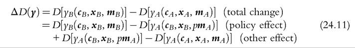

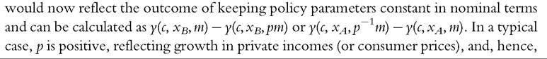 the policy effect would be negative (i.e., income-reducing). This is because a positive p implies higher benefit amounts and tax bands in the counterfactual scenario and translates into higher disposable incomes (for the same original incomes) compared to disposable incomes under tax-benefit rules when these are kept nominally constant. This has been studied, for example, by Immervoll (2005), Immervoll et al. (2006b) and Sutherland et al. (2008). It is also important to realize that if p is negative, meaning average original incomes (or prices) fall, and a tax-benefit system is kept nominally constant, then households’ tax burdens fall in relative terms.