Aggregate Demand and Aggregate Supply

model, but in fact the two models are equivalent. They are based on the same assumptions about economic behavior and price adjustment, and they give the same answers when used to analyze the effects of various shocks on the economy.

Explain the fundamentals and implications of the AD-AS model.

The Aggregate Demand Curve

The aggregate demand curve shows the relation between the aggregate quantity of goods demanded, C^d + I^d + G, and the price level, P. The aggregate demand curve slopes downward, as does the demand curve for a single product (apples, for example). Despite the superficial similarity between the AD curve and the demand curve for a specific good, however, there is an important difference between these two types of curves.

The reason that an increase in the price level, P, reduces the aggregate quan­tity of output demanded is illustrated in Figure 9.10. Recall that, for a given price level, the aggregate quantity of output that households, firms, and the government choose to demand is where the IS curve and the LM curve intersect. Suppose that the nominal money supply is M and that the initial price level is P₁. Then the real money supply is MP₁, and the initial LM curve is LM¹ in Fig. 9.10(a). The IS and LM¹ curves intersect at point E, where the amount of output that households, firms, and the government want to buy is Y₁. Thus we conclude that, when the price level is P₁, the aggregate amount of output demanded is Y₁.

Now suppose that the price level increases to P₂. With a nominal money sup­ply of M, this increase in the price level reduces the real money supply from M∕P₁ to M∕P₂. Recall (Summary table 13) that a decrease in the real money supply shifts the LM curve up and to the left, to LM². The IS and LM² curves intersect at point F, where the aggregate quantity of output demanded is Y₂. Thus the increase in the price level from P₁ to P₂ reduces the aggregate quantity of output demanded from Y₁ to Y₂.

This negative relation between the price level and the aggregate quantity of output demanded is shown as the downward-sloping AD curve in Fig.

FIGURE 9.10

Derivation of the aggregate demand curve

For a given price level, the aggregate quantity of output demanded is determined where the IS and LM curves intersect. If the price level, P, is P₁ and the initial LM curve is LM¹, the initial aggre­gate quantity of output demanded is Y₁, corre­sponding to point E in both (a) and (b). To derive the aggregate demand curve, we exam­ine what happens to the quantity of output demanded when the price level changes.

(a) An increase in the price level from P₁ to P₂ reduces the real money supply and shifts the LM curve up and to the left, from LM¹ to LM². Therefore the aggregate quantity of output demanded, represented by the intersection of the IS and LM curves, falls from Y₁ to Y₂.

(b) The increase in the price level from P₁ to P₂ reduces the aggregate quantity of output demanded from Y₁ at point E to Y₂ at point F, so the aggregate demand curve slopes downward.

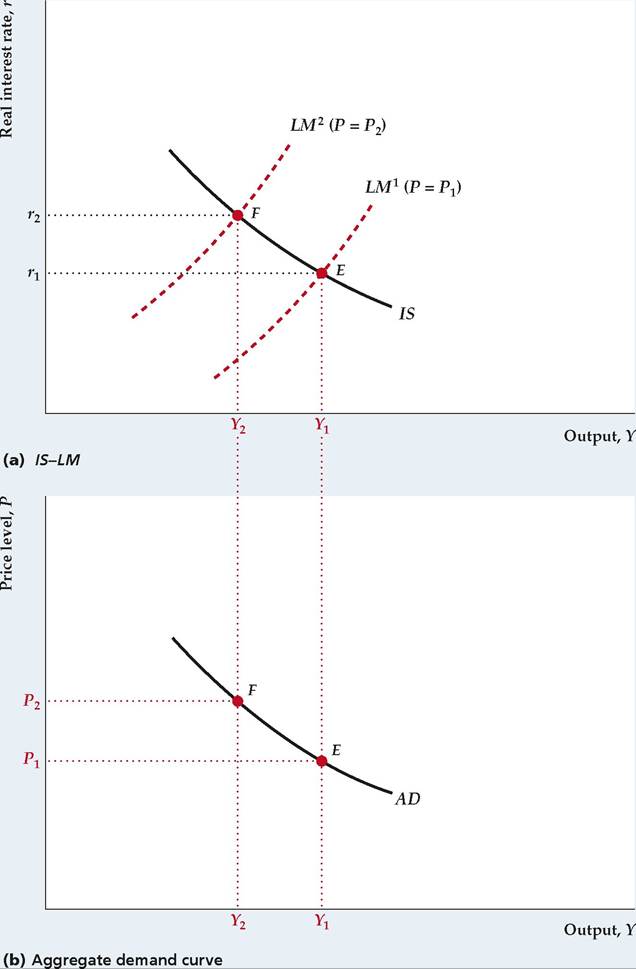
Points E and F in Fig. 9.10(b) correspond to points E and F in Fig. 9.10(a), respec­tively. The AD curve slopes downward because an increase in the price level reduces the real money supply, which shifts the LM curve up and to the left; the reduction in the real money supply increases the real interest rate, which reduces the demand for goods by households and firms.

Factors That Shift the AD Curve. The AD curve relates the aggregate quan­tity of output demanded to the price level. For a constant price level, any factor that changes the aggregate demand for output will cause the AD curve to shift, with increases in aggregate demand shifting the AD curve up and to the right and decreases in aggregate demand shifting it down and to the left. 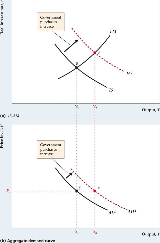Aggregate demand is determined by the intersection of the IS and LM curves, so we can also say that, holding the price level constant, any factor that causes the intersection of the IS curve and the LM curve to shift to the right raises aggregate demand and shifts the AD curve up and to the right.

An example of a factor that shifts the AD curve up and to the right, which we have considered before, is a temporary increase in government purchases. The effect of the increase in government purchases on the AD curve is illustrated in Figure 9.11. The initial IS curve, IS¹, intersects the LM curve at point E in Fig. 9.11(a) so that the initial aggregate quantity of output demanded is Y₁. As we have shown, a temporary increase in government purchases shifts the IS curve up and to the right to IS 2. With the price level held constant at its initial value of P₁, the intersec­tion of the IS and LM curves moves to point F so that the aggregate quantity of output demanded increases from Y₁ to Y2.

The shift of the AD curve resulting from the increase in government pur­chases is shown in Fig. 9.11(b). The increase in the aggregate quantity of output demanded at price level P₁ is shown by the movement from point E to point F. Because the increase in government purchases raises the aggregate quantity of output demanded at any price level, the entire AD curve shifts up and to the right, from AD¹ to AD 2. Other factors that shift the AD curve are listed in Summary table 14, and an algebraic derivation of the AD curve is presented in Appendix 9.B.

The Aggregate Supply Curve

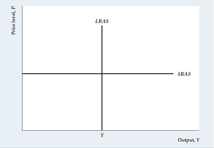
The aggregate supply curve shows the relationship between the price level and the aggregate amount of output that firms supply. Recall from the preview in Chapter 8 and our discussion of the IS-LM model that firms are assumed to behave differently in the short run than in the long run. The assumption is that prices remain fixed in the short run and that firms supply the quantity of output demanded at this fixed price level. Thus the short-run aggregate supply curve, or SRAS, is a horizontal line, as shown in Figure 9.12.

In the long run, prices and wages adjust to clear all markets in the economy. In particular, the labor market clears so that employment equals N, which is ⅛e~level of employment that maximizes firms' profits. When employment equals N, the aggregate amount of output supplied is the full-employment level, Y, which equals AF (K, N), regardless of the price level. In the long run, firms supply Y at any price level, so the long-run aggregate supply curve, or LRAS, is a vertical line at Y = Y, as shown in Fig. 9.12.

Factors That Shift the Aggregate Supply Curves. Any factor that increases the full-employment level of output, Y, shifts the long-run aggregate supply (LRAS) curve to the right, and any factor that reduces Y shifts the LRAS curve to

FIGURE 9.11

The effect of an increase in government purchases on the aggregate demand curve

(a) An increase in gov­ernment purchases shifts the IS curve up and to the right, from IS¹ to IS². At price level P₁, the aggregate quantity of output demanded increases from Y₁ to Y₂, as shown by the shift of the IS-LM intersection from point E to point F.

(b) Because the aggregate quantity of output demanded rises at any price level, the AD curve shifts up and to the right. Points E and F in (b) cor­respond to points E and F in (a), respectively.

the left. Thus any change that shifts the FE line to the right in the IS-LM diagram also shifts the LRAS curve to the right. For instance, an increase in the labor force raises the full-employment levels of employment and output, shifting the LRAS curve to the right.

SUMMARY 14

Factors That Shift the AD Curve

For a constant price level, any factor that shifts the intersection of the /S and LM curves to the right increases aggregate output demanded and shifts the AD curve up and to the right.

Factors that shift the /S curve up and to the right, and thus shift the AD curve up and to the right (see Summary table 12) include

■ an increase in expected future output;

■ an increase in wealth;

■ an increase in government purchases, G;

■ a reduction in taxes, T (assuming no Ricardian equivalence so that consumers respond by raising desired consumption);

■ an increase in the expected future TFP; and

■ a reduction in the effective tax rate on capital.

Factors that shift the LM curve down and to the right, and thus shift the AD curve up and to the right (see Summary table 13) include

■ an increase in the nominal money supply, M;

■ a rise in expected inflation, π^e;

■ a decrease in the nominal interest rate on money, i^m; and

■ any other change that reduces the real demand for money.

The short-run aggregate supply curve shifts whenever firms change their prices in the short run. Any factor, such as an increase in costs, that leads firms to increase prices in the short run will shift the SRAS curve up, and any factor that leads firms to decrease prices in the short run will shift the SRAS curve down.

FIGURE 9.12

The short-run and long-run aggregate supply curves

In the short run, firms supply the amount of output demanded at the fixed price, so the short­run aggregate supply (SRAS) curve is a hori­zontal line. In the long run, when the labor mar­ket clears, firms supply the full-employment level of output, Y, regardless of the price level. Thus the long-run aggregate supply (LRAS) curve is a vertical line at Y = Y.

Equilibrium in the AD-AS Model

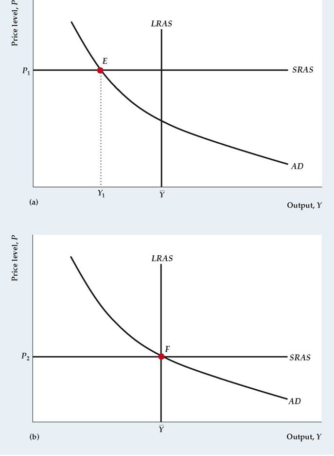
When we previewed the AD-AS model in Section 8.4, we introduced the distinc­tion between short-run equilibrium (equilibrium when the price level is fixed) and long-run equilibrium (equilibrium when the price level has fully adjusted). Short-run equilibrium is represented by the intersection of the AD and SRAS curves, as at point E in Figure 9.13(a). Notice that in this figure there is no com­mon point of intersection of all three curves. Long-run equilibrium is repre­sented by the intersection of the AD and LRAS curves, which is at point F in Fig. 9.13(b). The economy is also in short-run equilibrium at point F because point F is also at the intersection of the AD and SRAS curves. When the economy is in long-run equilibrium, output equals its full-employment level, Y. Long-run equilibrium is the same as general equilibrium because in long-run equilibrium all markets clear.

When the economy reaches general, or long-run, equilibrium, all three curves—AD, SRAS, and LRAS—intersect at a common point, as in Fig. 9.13(b). This condition isn't a coincidence. As with the IS curve, the LM curve, and the FE line, strong economic forces lead the economy to arrive eventually at a common point of intersection of the three curves. Indeed, the forces leading the AD, SRAS, and LRAS curves to intersect at a common point are the same as the forces lead­ing the IS curve, the LM curve, and FE line to intersect at a common point. To illustrate, we use the AD-AS framework to examine the effects on the economy of an increase in the money supply, which we previously analyzed with the IS-LM model.

Monetary Neutrality in the AD-AS Model

Suppose that the economy is initially in equilibrium at point E in Figure 9.14, where the level of output is Y and the price level is P₁, and that the money supply then increases by 10%. In the IS-LM model an increase in the money supply shifts the LM curve down and to the right, raising the aggregate quantity of output demanded at any particular price level. Thus an increase in the money supply also shifts the AD curve up and to the right, from AD¹ to AD².

Moreover, when the money supply rises by 10%, points on the new AD curve are those for which the price level is 10% higher at each level of output demanded. To see why, compare points E and H. Because H lies on AD² and E lies on AD¹, the nominal money supply, M, is 10% higher at H than at E. However, the aggregate quantity of output demanded is the same (Y) at H and E. The aggregate quantity of output demanded can be the same at H and E only if the real money supply, M∕P, which determines the position of the LM curve and hence the aggregate quantity of output demanded, is the same at H and E. With the nominal money supply 10% higher at H, for the real money supply to be the same at the two points the price level at H must be 10% higher than at E. Therefore P₂ is 10% higher than P₁. Indeed, for every level of output, the price level is 10% higher on AD² than on AD¹.

In the short run, the price level remains fixed, and the increase in the nominal money supply shifts the aggregate demand curve from AD¹ to AD². Thus the short-run equilibrium moves from point E to point F (which corresponds to move­ment from point E to point F in the IS-LM diagram in Fig. 9.9a). Thus in the short

FIGURE 9.13

Equilibrium in the AD-AS model

(a) Short-run equilibrium is represented by the intersection of the AD and SRAS curves at point E. At short-run equilib­rium, the price level is fixed at P₁ and firms meet demand at those prices.

(b) Long-run equilib­rium, which occurs after the price level has fully adjusted (declined) from P₁ to P₂, is represented by the intersection of the AD and LRAS curves at point P. Long-run equi­librium is the same as general equilibrium because in long-run equi­librium all markets clear.

run the increase in the nominal money supply increases output from Y to Y₂, caus­ing an economic boom.

However, the economy won't remain at point P indefinitely. Because the amount of output, Y₂, is higher than the profit-maximizing level of output, Y, firms will eventually increase their prices. Rising prices cause the short-run

FIGURE 9.14

Monetary neutrality in the AD-AS framework

If we start from general equilibrium at point E, a 10% increase in the nominal money supply shifts the AD curve up and to the right from AD¹ to AD 2. The points on the new AD curve are those for which the price level is 10% higher at each level of output demanded because a 10% increase in the price level is needed to keep the real money supply, and thus the aggregate quantity of output demanded, unchanged. In the new short-run equilibrium at point F, the price level is unchanged, and output is higher than its full­employment level. In the new long-run equilib­rium at point H, output is unchanged at Y, and the price level P₂ is 10% higher than the initial price level P₁. Thus money is neutral in the long run.

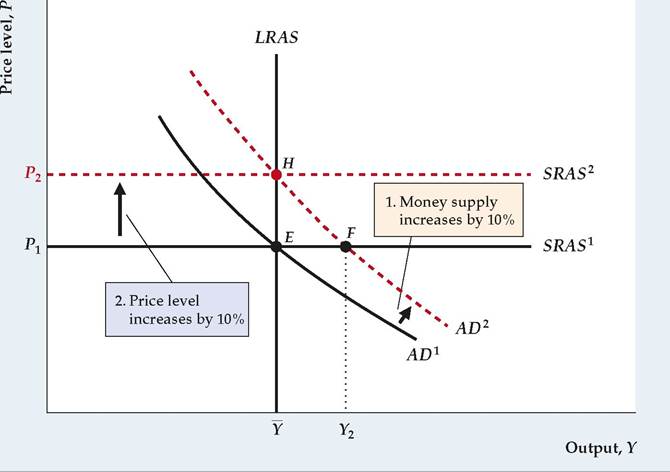
aggregate supply curve to shift up from SRAS¹. Firms will increase their prices until the quantity of output demanded falls to the profit-maximizing level of output, Y. The new long-run equilibrium is represented by point H, where the AD curve, the LRAS curve, and the new short-run aggregate supply curve, or SRAS 2, all intersect. In the new long-run equilibrium, the price level has increased by 10%, which is the same amount that the nominal money supply has increased. Output is the same in the new long-run equilibrium at point H as at point E. Thus we conclude that money is neutral in the long run, as we did when using the IS-LM model.

Our analysis highlights the distinction between the short-run and long-run effects of an increase in the money supply, but it leaves open the crucial question of how long it takes the economy to reach long-run equilibrium. As we have emphasized in both Chapter 8 and this chapter, classical and Keynesian econo­mists have very different answers to this question. Classical economists argue that the economy reaches its long-run equilibrium quickly. Indeed, in its strictest form, the classical view is that the economy reaches long-run equilibrium almost imme­diately, so that the long-run aggregate supply (LRAS) curve is the only aggregate supply curve that matters [the short-run aggregate supply (SRAS) curve is irrele­vant]. However, Keynesians argue that the economy may take years to reach long- run equilibrium and that in the meantime output will differ from its full­employment level. We elaborate on these points of view in Chapter 10, which is devoted to the classical model, and in Chapter 11, which is devoted to the Keynesian model.