Price Adjustment and the Attainment of General Equilibrium

Discuss the role of price adjustment in achieving general equilibrium.

We now explain the economic forces that lead the price level to change and shift the LM curve until it passes through the intersection of the IS curve and the FE line.

To illustrate the adjustment process, let's use the complete IS-LM model to consider what happens to the economy if the nominal money supply increases. This analysis allows us to discuss monetary policy (the control of the money sup­ply) and to introduce some ongoing controversies about the effects of monetary policy on the economy.

The Effects of a Monetary Expansion

Suppose that the central bank decides to raise the nominal money supply, M, by 10%. For now we hold the price level, P, constant so that the real money supply, M∣P, also increases by 10%. What effects will this monetary expansion have on the economy? Figure 9.9 helps us answer this question with the complete IS-LM model. The two parts of Fig. 9.9 show the sequence of events involved in the analysis. For simplicity, suppose that the economy initially is in general equilibrium so that in Fig. 9.9(a) the IS curve, the FE line, and the initial LM curve, LM¹, all pass through the general equilibrium point, E. At E output equals its full-employment value of 1000, and the real interest rate is 5%. Both the IS and LM curves pass through E, so we know that 5% is the market-clearing real interest rate in both the goods and asset markets. For the moment the price level, P, is fixed at its initial level of 100.

The 10% increase in the real supply of money, M∣P, doesn't shift the IS curve or the FE line because, with output and the real interest rate held constant, a

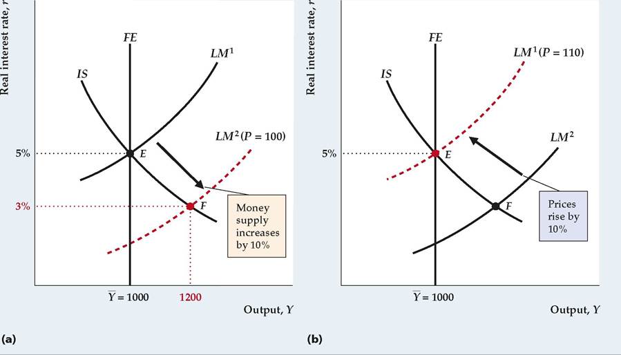
FIGURE 9.9

Effects of a monetary expansion

(a) The economy is in general equilibrium at point E.

(b) Because aggregate demand exceeds full-employment output at point F, firms raise prices. A 10% rise in P, from 100 to 110, restores the real money supply to its original level and shifts the LM curve back to its original position at LM¹. This returns the economy to point E, where output again is at its full-employment level of 1000, but the price level has risen 10% from 100 to 110.

change in MP doesn't affect desired national saving, desired investment, labor demand, labor supply, or productivity. However, Fig. 9.5 showed that an increase in the real money supply does shift the LM curve down and to the right, which we show here as a shift of the LM curve from LM¹ to LM², in Fig. 9.9(a). The LM curve shifts down and to the right because, at any level of output, an increase in the money supply lowers the real interest rate needed to clear the asset market.

Note that, after the LM curve has shifted down to LM², there is no point in Fig. 9.9(a) at which all three curves intersect. In other words, the goods market, the labor market, and the asset market no longer are simultaneously in equilibrium. We now must make some assumptions about how the economy behaves when it isn't in general equilibrium.

Of the three markets in the IS-LM model, the asset market (represented by the LM curve) undoubtedly adjusts the most quickly because financial markets can respond within minutes to changes in economic conditions.

Immediately after the increase in the nominal money supply, therefore, the economy is out of general equilibrium with the level of output and the real inter­est rate represented by point F in Fig. 9.9(a), where the new LM curve, LM², inter­sects the IS curve. At F, output (1200) is higher and the real interest rate (3%) is lower than at the original general equilibrium, point E. We refer to F, the point at which the economy comes to rest before any adjustment occurs in the price level, as the short-run equilibrium point. (Although we refer to F as a short-run equilib­rium point, keep in mind that only the asset and goods markets are in equilibrium there—the labor market isn't.)

In economic terms, why does the increase in the money supply shift the econ­omy to point F? The sequence of events can be described as follows: After the increase in the money supply, holders of wealth are holding more money in their portfolios than they desire at the initial values of output and the real interest rate. To bring their portfolios back into balance, they will try to use their excess money to buy nonmonetary assets. However, as holders of wealth bid for nonmonetary assets, they put upward pressure on the prices of those assets, which reduces their interest rate. Thus after an increase in the money supply, wealth-holders' attempts to achieve their desired mix of money and nonmonetary assets cause the interest rate to fall.

The drop in the real interest rate isn't the end of the story, however. Because the lower real interest rate increases the demand by households for consumption, C^d, and the demand by firms for investment, I^d, the aggregate demand for goods rises. Here we make a fundamental assumption, to which we return shortly: When demanders increase their spending on goods, firms are willing (at least temporar­ily) to produce enough to meet the extra demand for their output. After the decline in the real interest rate raises the aggregate demand for goods, therefore, we assume that firms respond by increasing production, leading to higher output at the short-run equilibrium point, F.

To summarize, with the price level constant, an increase in the nominal money supply takes the economy to the short-run equilibrium point, F, in Fig. 9.9(a), at which the real interest rate is lower and output is higher than at the initial general equilibrium point, E. We made two assumptions: (1) When the economy isn't in general equilibrium, the economy's short-run equilibrium occurs at the intersec­tion of the IS and LM curves; and (2) when the aggregate demand for goods rises, firms are willing (at least temporarily) to produce enough extra output to meet the expanded demand.

The Adjustment of the Price Level. So far we have simply taken the price level, P, as fixed. In reality, prices respond to conditions of supply and demand in the economy. The price level, P, refers to the price of output (goods), so to think about how prices are likely to adjust in this example, let's reconsider the effects of the increase in the money supply on the goods market.

In Fig. 9.9(a), the short-run equilibrium point, F, lies on the IS curve, implying that the goods market is in equilibrium at that point with equal aggregate quanti­ties of goods supplied and demanded. Recall our assumption that firms are will­ing to meet any increases in aggregate demand by producing more. In that sense, then, the aggregate quantity of goods supplied equals the aggregate quantity of goods demanded.

At point F the aggregate demand for goods exceeds firms' desired supply of output, Y, so we can expect firms to begin raising their prices, causing the price level, P, to rise. With the nominal money supply, M, set by the central bank, an increase in the price level, P, lowers the real money supply, M/P, which in turn causes the LM curve to shift up and to the left. Indeed, as long as the aggregate quantity of goods demanded exceeds what firms want to supply, prices will keep rising. Thus the LM curve will keep shifting up and to the left until the aggregate quantity of goods demanded equals full-employment output. Aggregate demand equals full-employment output only when the LM curve has returned to its initial position, LM¹ in Fig. 9.9(b), where it passes through the original general equilib­rium point, E. At E all three markets of the economy again are in equilibrium, with output at its full-employment level.

Compare Fig. 9.9(b) to the initial situation in Fig. 9.9(a) and note that after the adjustment of the price level the 10% increase in the nominal money supply has had no effect on output or the real interest rate. Employment also is unchanged from its initial value, as the economy has returned to its original level of output. However, as a result of the 10% increase in the nominal money supply, the price level is 10% higher (so that P = 110).

Note that, because in general equilibrium the price level has risen by 10% but real economic variables are unaffected, all nominal economic variables must also rise by 10%. In particular, for the real wage to have the same value after prices have risen by 10% as it did before, the nominal wage must rise by 10%. Thus the return of the economy to general equilibrium requires adjustment of the nominal wage (the price of labor) as well as the price of goods.

Trend Money Growth and Inflation. In Fig 9.9 we analyzed the effects of a one­time 10% increase in the nominal money supply, followed by a one-time 10% adjust­ment in the price level. In reality, in most countries the money supply and the price level grow continuously. Our framework easily handles this situation. Suppose that in some country both the nominal money supply, M, and the price level, P, are grow­ing steadily at 7% per year, which implies that the real money supply, MP, is con­stant. The LM curve depends on the real money supply, M∣P, so in this situation the LM curve won't shift, even though the nominal money supply and prices are rising.

Now suppose that for one year the money supply of this country is increased an additional 3%—for a total of 10%—while prices rise 7%. Then the real money supply, M∕P, grows by 3% (10% minus 7%), and the LM curve shifts down and to the right. Similarly, if for one year the nominal money supply increased by only 4%, with inflation still at 7% per year, the LM curve would shift up and to the left, reflecting the 3% drop (-3% = 4% — 7%) in the real money supply.

This example illustrates that changes in M or P relative to the expected or trend rate of growth of money and inflation (7% in this example) shift the LM curve. Thus when we analyze the effects of "an increase in the money supply," we have in mind an increase in the money supply relative to the expected, or trend, rate of money growth (for example, a rise from 7% to 10% growth for one year); by a "decrease in the money supply," we mean a drop relative to a trend rate (such as a decline from 7% to 4% growth in money). Similarly, if we say something like "the price level falls to restore general equilibrium," we don't necessarily mean that the price level literally falls but only that it rises by less than its trend or expected rate of growth would suggest.

Classical Versus Keynesian Versions of the IS-LM Model

Our diagrammatic analysis of the effects of a change in the money supply high­lights two questions that are central to the debate between the classical and Keynesian approaches to macroeconomics: (1) How rapidly does the economy reach general equilibrium? and (2) What are the effects of monetary policy on the economy? We previewed the first of these questions in Section 8.4, using the AD-AS model. Now we examine both questions, using the IS-LM model.

Price Adjustment and the Self-Correcting Economy. In our analysis of the effects of a monetary expansion, we showed that the economy is brought into general equilibrium by adjustment of the price level. In graphical terms, if the intersection of the IS and LM curves lies to the right of the FE line—so that the aggregate quantity of goods demanded exceeds full-employment output, as at point F in Fig. 9.9(a)— the price level will rise. The increase in P shifts the LM curve up and to the left, reducing the quantity of goods demanded, until all three curves intersect at the general equilibrium point, as in Fig. 9.9(b). Similarly, if the IS-LM intersection lies to the left of the full-employment line—so that desired spending on goods is below firms' profit-maximizing level of output—firms will cut prices. A decrease in the price level raises the real money supply and shifts the LM curve down and to the right, until all three curves again intersect, returning the economy to general equilibrium. In summary, in a short-run equilibrium, output and the real interest rate are endogenous variables in the model, and the price level is fixed and thus exogenous. In general equilibrium, all three variables (output, the real interest rate, and the price level) are endogenous and determined by the model.

There is little disagreement about the idea that, after some sort of economic dis­turbance, price level adjustments will eventually restore the economy to general equi­librium. However, as discussed in Section 8.4, the speed at which this process takes place is a controversial issue in macroeconomics. Under the classical assumption that prices are flexible, the adjustment process is rapid. When prices are flexible, the economy is effectively self-correcting, automatically returning to full employment after a shock moves it away from general equilibrium.^{[158] [159] Indeed, if firms respond to increased demand by raising prices rather than by temporarily producing more (as we earlier assumed), the adjustment process would be almost immediate.}

According to the opposing Keynesian view, however, sluggish adjustment of prices (and of wages, the price of labor) might prevent general equilibrium from being attained for a much longer period, perhaps even several years. While the economy is not in general equilibrium, Keynesians argue, output is determined by the level of aggregate demand, represented by the intersection of the IS and LM curves; the economy is not on the FE line, and the labor market is not in equilib­rium. This assumption of sluggish price adjustment, and the consequent disequi­librium in the labor market, distinguishes the Keynesian version of the IS-LM model from the classical version.

Monetary Neutrality. Closely related to the issue of how fast the economy reaches general equilibrium is the question of how a change in the nominal money supply affects the economy. We showed that, after the economy reaches its general equilibrium, an increase in the nominal money supply has no effect on real vari­ables such as output, employment, or the real interest rate but raises the price level. Economists say that there is monetary neutrality, or simply that money is neutral, if a change in the nominal money supply changes the price level propor­tionally but has no effect on real variables. Our analysis shows that, after the com­plete adjustment of prices, money is neutral in the IS-LM model.

The practical relevance of monetary neutrality is much debated by classicals and Keynesians. The basic issue again is the speed of price adjustment. In the classical view a monetary expansion is rapidly transmitted into prices and has, at most, a tran­sitory effect on real variables; that is, the economy moves quickly from the general­equilibrium situation shown in Fig. 9.9(a) to the general-equilibrium situation shown in Fig. 9.9(b), spending little time out of general equilibrium at point F in Fig. 9.9(a). Keynesians agree that money is neutral after prices fully adjust but believe that, because of slow price adjustment, the economy may spend a long time in disequilib­rium. During this period the increased money supply causes output and employ­ment to rise and the real interest rate to fall (compare point F to point E in Fig. 9.9a).

In brief, Keynesians believe in monetary neutrality in the long run (after prices adjust) but not in the short run. Classicals are more accepting of the view that money is neutral even in the relatively short run. We return to the issue of mone­tary neutrality when we develop the classical and Keynesian models of the busi­ness cycle in more detail in Chapters 10 and 11.

9.5