General Equilibrium in the Complete IS-LM Model

Describe the conditions necessary for general equilibrium using the IS-LM model.

The next step is to put the labor market, the goods market, and the asset market together and examine the equilibrium of the economy as a whole.

■ the full-employment, or FE, line, along which the labor market is in equilibrium;

■ the IS curve, along which the goods market is in equilibrium; and

■ the LM curve, along which the asset market is in equilibrium.

The three curves intersect at point E, indicating that all three markets are in equilibrium at that point. Therefore E represents a general equilibrium and, because it is the only point that lies on all three curves, the only general equilibrium for this economy.

Although point E obviously is a general equilibrium point, not so clear is which forces, if any, act to bring the economy to that point. To put it another way, although the IS curve and FE line must intersect somewhere, we haven't explained why the LM curve must pass through that same point. In Section 9.5 we discuss the economic forces that lead the economy to general equilibrium. There we show that (1) the general equilibrium of the economy always occurs at the intersection of the IS curve and the FE line; and (2) adjustments of the price level cause the LM curve to shift until it passes through the general equilibrium point defined by the intersection of the IS curve and the FE line. Before discussing the details of this adjustment process, however, let's consider an example that illustrates the use of the complete IS-LM model.

FIGURE 9.7

General equilibrium in the IS-LM model

The economy is in gen­eral equilibrium when quantities supplied equal quantities demanded in every market.

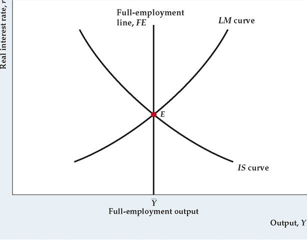
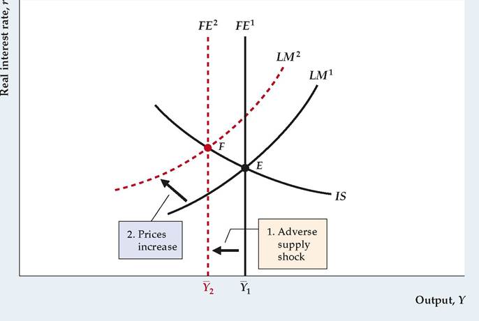
FIGURE 9.8

Effects of a temporary adverse supply shock Initially, the economy is in general equilibrium at point E, with output at its full-employment level, Y₁. A temporary adverse supply shock reduces full-employment output from Y₁ to Y₂ and shifts the FE line to the left from FE¹ to FE². The new general equilibrium is represented by point F, where FE² intersects the unchanged IS curve. The price level increases and shifts the LM curve up and to the left, from LM¹ to LM², until it passes through F. At the new general equilibrium point, F, output is lower, the real interest rate is higher, and the price level is higher than at the original general equilib­rium point, E.

Applying the IS-LM Framework: A Temporary Adverse Supply Shock

An economic shock relevant to business cycle analysis is an adverse supply shock. Specifically, suppose that (because of bad weather or a temporary increase in oil prices) the productivity parameter, A, in the production function drops temporarily.^{* [154] [155]} We can use the IS-LM model to analyze the effects of this shock on the general equilibrium of the economy and the general equilibrium values of economic vari­ables such as the real wage, employment, output, the real interest rate, the price level, consumption, and investment.

Suppose that the economy is initially in general equilibrium at point E in Figure 9.8, where the initial FE line, FE¹, IS curve, and LM curve, LM¹, for this economy intersect. To determine the effects of a temporary supply shock on the general equilibrium of this economy, we must consider how the temporary drop in productivity A affects the positions of the FE line and the IS and LM curves.

The FE line describes equilibrium in the labor market. Hence to find the effect of the supply shock on the FE line we must first look at how the shock affects labor supply and labor demand. In Chapter 3 we demonstrated that an adverse supply shock reduces the marginal product of labor and thus shifts the labor demand curve down (see Fig. 3.10). Because the supply shock is temporary, we assume that

The FE line shifts only to the degree that full-employment output, Y, changes. Does Y change? Yes. Recall from Chapter 3 that an_adverse supply shock reduces full-employment output, Y, which equals AF (K, N), for two reasons: (1) As we just mentioned, the supply shock reduces the equilibrium level of employment, N, which lowers the amount of output that can be produced; and (2) the drop in pro­ductivity A directly reduces the amount of output produced by any combination of capital and labor. The reduction in Y is represented by a shift to the left of the FE line, from FE¹ to FE² in Fig. 9.8.

Now consider the effects of the temporary adverse supply shock on the IS curve. Recall that we derived the IS curve by changing the level of current output in the saving-investment diagram (Fig. 9.2) and finding for each level of current output the real interest rate for which desired saving equals desired investment. A temporary adverse supply shock reduces current output but doesn't change any other factor affecting desired saving or investment (such as wealth, expected future income, or the future marginal product of capital). Therefore a temporary supply shock is just the sort of change in current output that we used to trace out the IS curve. We conclude that a temporary adverse supply shock is a movement along the IS curve, not a shift of the IS curve, leaving it unchanged.^[156]

Finally, we consider the LM curve. A temporary supply shock has no direct effect on the demand or supply of money and thus doesn't shift the LM curve.

We now look for the new general equilibrium of the economy. In Fig. 9.8, there is no point at which FE² (the new FE line), IS, and LM¹ all intersect. As we mentioned—and demonstrate in Section 9.5—when the FE line, the IS curve, and the LM curve don't intersect at a common point, the LM curve shifts until it passes through the intersection of the FE line and IS curve. This shift in the LM curve is caused by a change in the price level, P, which changes the real money supply, MP, and thus affects the equilibrium of the asset market. As Fig. 9.8 shows, to restore general equilibrium at point F, the LM curve must shift up and to the left, from LM¹ to LM². For it to do so, the real money supply M/P must fall (see Summary table 13) and thus the price level, P, must rise. We infer (although we haven't yet given an economic explanation) that an adverse supply shock will cause the price level to rise.

What is the effect of a temporary supply shock on the inflation rate, as distinct from the price level? As the inflation rate is the growth rate of the price level, dur­ing the period in which prices are rising to their new, higher level, a burst of infla­tion will occur. However, after the price level stabilizes at its higher value (and is no longer rising), inflation will subside. Thus a temporary supply shock should cause a temporary, rather than a permanent, increase in the rate of inflation.

Let's pause and review our results.

1. As we had already shown in Chapter 3, a temporary adverse supply shock lowers the equilibrium values of the real wage and employment.

2. Comparing the new general equilibrium, point F, to the old general equilib­rium, point E, in Fig. 9.8, we see that the supply shock lowers output and raises the real interest rate.

3. The supply shock raises the price level and causes a temporary burst of inflation.

4. Because in the new general equilibrium the real interest rate is higher and output is lower, consumption must be lower than before the supply shock.

In the Application "The Oil Price Shock of 2008," we check out how well our model explains the historical behavior of the economy. Note that economic models, such as the IS-LM model, also are used extensively in forecasting economic condi­tions ("In Touch with Data and Research: Econometric Models and Macroeconomic Forecasts for Monetary Policy Analysis").

Application

The Oil Price Shock of 2008

In 2008, oil prices swung wildly. In the first half of the year, oil prices (measured by the price of a barrel of West Texas Intermediate Grade Crude Oil) rose from $96 on January 1 (and had been as low as $51 in January 2007) to a peak of $145 in July. A supply shock of this magnitude would normally have an adverse effect on output, employment, and investment, of course. But when combined with the housing crisis and financial crisis that developed in 2008, the declines in output, employ­ment, and investment were extremely steep as the economy entered the greatest recession since the Great Depression of the 1930s.

Our theory predicts that an adverse supply shock like the oil price shock of 2008 will cause real interest rates to rise. However, to combat the housing crisis and later the financial crisis that year, the Federal Reserve reduced nominal inter­est rates dramatically, especially when the financial crisis worsened in September 2008. As a result, real interest rates also declined, and in many cases became negative.

As the financial crisis spread across the globe, worldwide demand for oil fell sharply and the price of oil declined from $145 in July to $30 in mid-December. Thus the adverse supply shock became a beneficial supply shock. But of course, the damage to the economy from the housing crisis and financial crisis dominated the beneficial effects of lower oil prices.

In Touch with Data and Research

Econometric Models and Macroeconomic Forecasts for Monetary Policy Analysis

The IS-LM model developed in this chapter is a relatively simple example of a macroeconomic model.

A common use of macroeconomic models is to help economists forecast the course of the economy. In general, using a macroeconomic model to obtain quan­titative economic forecasts involves three steps. First, numerical values for the parameters of the model (such as the income elasticity of money demand) must be obtained. In econometric models, these values are estimated through statistical analyses of the data. Second, projections must be made of the likely behavior of relevant exogenous variables, or variables whose values are not determined within the model. Examples of exogenous variables include policy variables (such as government spending and the money supply), oil prices, and changes in produc­tivity. Third, based on the expected path of the exogenous variables and the model parameters, the model can be solved (usually on a computer) to give forecasts of variables determined within the model (such as output, employment, and interest rates). Variables determined within the model are endogenous variables.^[157]

Although a relatively simple model like the IS-LM model developed in this chapter could be used to create real forecasts, the results probably would not be very good. Because real-world economies are complex, macroeconomic models actually used in forecasting tend to be much more detailed than the IS-LM model presented here. For example, the Federal Reserve Board has long had such a model in place for analyzing the economy and for developing forecasts for use in monetary policy.

In 1996, the Federal Reserve Board produced a new model for policy analysis and forecasting, known as the FRB/US model, and has been continually upgrading the model since then. FRB/US was based on a previous model known as the MPS model, which was developed closely from the theoretical IS-LM model but with hundreds of equations representing different industries and sectors of the economy. The new FRB/US model differed from the old MPS model in a number of ways: It featured a much better ability to handle people's expectations about the future values of inflation and other variables, improved modeling of people's and firms' reactions to economic shocks, and used newer statistical techniques to estimate the model. The model is also available for anyone to use on the Federal Reserve Board's website at www.federalreserve.gov/econres/us-models-about.htm.

The staff economists at the Federal Reserve Board now use the model as a workhorse for policy analysis. They apply results from the model to analyze alternative monetary policy scenarios—for example, what would happen to the economy over the next two years if the Fed raised the federal funds interest rate to 3%, compared with a scenario in which the rate were set at a lower level, such as 0.25%. This analysis gives policymakers an idea of how policy affects the economy and what are the likely outcomes of policy choices.

The model contains three main sectors of the economy, just as the IS-LM model does: households, firms, and financial markets. Households supply labor, as we discussed in Section 3.3, and decide how much to consume and save, as we saw in Section 4.1 and Appendix 4.A. Firms maximize their profits, choos­ing appropriate levels of investment, as we discussed in Section 4.2, and demand labor, as we saw in Section 3.2. Firms' and households' demand and supply of financial assets determine equilibrium in the financial markets, as we discussed in Chapter 7. The model is solved with general equilibrium concepts, as we showed in Sections 3.4 for labor markets, 4.3 for goods markets, and 7.4 for asset markets. Overall economic growth is governed by the principles discussed in Chapter 6. Other assumptions of the model are based on new Keynesian theory, as we will discuss in Chapter 11.

Although the model is quite detailed, no macro model is able to provide accu­rate forecasts without some human judgment. So, to produce the forecasts that the Fed uses internally in its Tealbook (formerly Greenbook) publication, the FRB/US model forecasts are analyzed by the staff at the Federal Reserve Board and are often modified somewhat before being presented to monetary policymakers. The judgment of the staff economists who are experts in various sectors of the econ­omy is an important input into the Tealbook forecasts. Research suggests that this method of producing forecasts produces better results than private-sector fore­casts, especially when forecasting inflation.¹⁰

¹⁰See Christina Romer and David Romer, “Federal Reserve Information and the Behavior of Interest Rates,” American Economic Review (June 2000), pp. 429-457; and Christopher Sims, “The Role of Models and Probabilities in the Monetary Policy Process,” Brookings Papers on Economic Activity (2:2002), pp. 1-62.

9.4