The LM Curve: Asset Market Equilibrium
Discuss factors that affect the LM curve, which represents equilibrium in the asset market.
The Interest Rate and the Price of a Nonmonetary Asset
The price of a nonmonetary asset, such as a government bond, is what a buyer has to pay for it.
Its price is closely related to the interest rate that it pays (sometimes called its yield). To illustrate this relationship with an example, let's consider a bond that matures in one year. At maturity, we assume, the bondholder will redeem it and receive $10,000; the bond doesn't pay any interest before it matures.[152] Suppose that this bond can be purchased now for $9615. At this price, over the coming year the bond will increase in value by $385 ($10,000 — $9615), or approximately 4% of its current price of $9615. Therefore the nominal interest rate on the bond, or its yield, is 4% per year.Now suppose that for some reason the current price of a $10,000 bond that matures in one year drops to $9524. The increase in the bond's value over the coming year will be $476 ($10,000 — $9524), or approximately 5% of the purchase price of $9524. Therefore, when the current price of the bond falls to $9524, the nominal interest rate on the bond increases to 5% per year. More generally, for the promised schedule of payments on a bond or other nonmonetary asset, the higher the price of the asset, the lower the nominal interest rate that the asset pays. Thus a media report that, in yesterday's trading, the bond market "strengthened" (bond prices rose), is equivalent to saying that nominal interest rates fell.
We have just indicated why the price of a nonmonetary asset and its nominal interest rate are negatively related. For a given expected rate of inflation, πe, movements in the nominal interest rate are matched by equal movements in the real interest rate, so the price of a nonmonetary asset and its real interest rate are also inversely related.
This relationship is a key to deriving the LM curve and explaining how the asset market comes into equilibrium.The Equality of Money Demanded and Money Supplied
To derive the LM curve, which represents asset market equilibrium, we recall that the asset market is in equilibrium only if the quantity of money demanded equals the currently available money supply. We depict the equality of money supplied and demanded using the money supply-money demand diagram, shown in Figure 9.4(a). The real interest rate is on the vertical axis and money, measured in real terms, is on the horizontal axis.[153] The MS line shows the economy's real money supply, M∕P. The nominal money supply, M, is set by the central bank. Thus for a given price level, P, the real money supply, M∕P, is a fixed number and the MS line is vertical. For example, if M = 2000 and P = 2, the MS line is vertical at M∣P = 1000.
Real money demand at two different levels of income, Y, is shown by the two MD curves in Fig. 9.4(a). Recall from Chapter 7 that for a given value of the expected rate of inflation, πe, a higher real interest rate, r, increases the relative attractiveness of nonmonetary assets and causes holders of wealth to demand less money. Thus the money demand curves slope downward. The money demand curve, MD, for Y = 4000 shows the real demand for money when output is 4000;
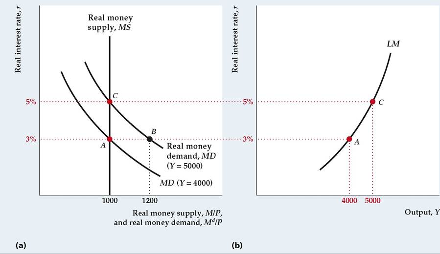
FIGURE 9.4
Deriving the LM curve
(a) The curves show real money demand and real money supply. Real money supply is fixed at 1000. When output is 4000, the real money demand curve is MD (Y = 4000); the real interest rate that clears the asset market is 3% (point A). When output is 5000, more money is demanded at the same real interest rate, so the real money demand curve shifts to the right to MD (Y = 5000). In this case the real interest rate that clears the asset market is 5% (point C).
(b) The graph shows the corresponding LM curve. For each level of output, the LM curve shows the real interest rate that clears the asset market. Thus when output is 4000, the LM curve shows that the real interest rate that clears the asset market is 3% (point A). When output is 5000, the LM curve shows a market-clearing real interest rate of 5% (point C). Because higher output raises money demand, and thus raises the real interest rate that clears the asset market, the LM curve slopes upward.
similarly, the MD curve for Y = 5000 shows the real demand for money when output is 5000. Because an increase in income increases the amount of money demanded at any real interest rate, the money demand curve for Y = 5000 is farther to the right than the money demand curve for Y = 4000.
Graphically, asset market equilibrium occurs at the intersection of the money supply and money demand curves, where the real quantities of money supplied and demanded are equal. For example, when output is 4000, so that the money demand curve is MD (Y = 4000), the money demand and money supply curves intersect at point A in Fig. 9.4(a). The real interest rate at A is 3%. Thus when output is 4000, the real interest rate that clears the asset market (equalizes the quantities of money supplied and demanded) is 3%. At a real interest rate of 3% and an output of 4000, the real quantity of money demanded by holders of wealth is 1000, which equals the real money supply made available by the central bank at the given price level.
What happens to the asset market equilibrium if output rises from 4000 to 5000? People need to conduct more transactions, so their real money demand increases at any real interest rate. As a result, the money demand curve shifts to the right, to MD (Y = 5000). If the real interest rate remained at 3%, the real quantity of money demanded would exceed the real money supply. At point B in Fig. 9.4(a) the real quantity of money demanded is 1200, which is greater than the real money supply of 1000.
To restore equality of money demanded and supplied and thus bring the asset market back into equilibrium, the real interest rate must rise to 5%. When the real interest rate is 5%, the real quantity of money demanded declines to 1000, which equals the fixed real money supply (point C in Fig. 9.4a).How does an increase in the real interest rate eliminate the excess demand for money, and what causes this increase in the real interest rate? Recall that the prices of nonmonetary assets and the interest rates they pay are negatively related. At the initial real interest rate of 3%, the increase in output from 4000 to 5000 causes people to demand more money (the MD curve shifts to the right in Fig. 9.4a). To satisfy their desire to hold more money, people will try to sell some of their nonmonetary assets for money. But when people rush to sell a portion of their nonmonetary assets, the prices of these assets will fall, which means that the real interest rates on these assets rise. Thus it is the public's attempt to increase its holdings of money by selling nonmonetary assets that causes the real interest rate to rise.
Because the real supply of money in the economy is fixed, the public as a whole cannot increase the amount of money it holds. As long as people attempt to do so by selling nonmonetary assets, the real interest rate will continue to rise. But the increase in the real interest rate paid by nonmonetary assets makes those assets more attractive relative to money, reducing the real quantity of money demanded (here the movement is along the MD curve for Y = 5000, from point B to point C in Fig. 9.4a). The real interest rate will rise until the real quantity of money demanded again equals the fixed supply of money and restores asset market equilibrium. The new asset market equilibrium is at C, where the real interest rate has risen from 3% to 5%.
The preceding example shows that when output rises, increasing real money demand, a higher real interest rate is needed to maintain equilibrium in the asset market.
In general, the relationship between output and the real interest rate that clears the asset market is expressed graphically by the LM curve. For any level of output, the LM curve shows the real interest rate for which the asset market is in equilibrium, with equal quantities of money supplied and demanded. The term LM comes from the asset market equilibrium condition that the real quantity of money demanded, as determined by the real money demand function, L, must equal the real money supply, M∕P.The LM curve corresponding to our numerical example is shown in Fig. 9.4(b), with the real interest rate, r, on the vertical axis and output, Y, on the horizontal axis. Points A and C lie on the LM curve. At A, which corresponds to point A in the money supply-money demand diagram of Fig. 9.4(a), output, Y, is 4000 and the real interest rate, r, is 3%. Because A lies on the LM curve, when output is 4000 the real interest rate that clears the asset market is 3%. Similarly, because C lies on the LM curve, when output is 5000 the real interest rate that equalizes money supplied and demanded is 5%; this output-real interest rate combination corresponds to the asset market equilibrium at point C in Fig. 9.4(a).
Figure 9.4(b) illustrates the general point that the LM curve always slopes upward from left to right. It does so because increases in output, by raising money demand, also raise the real interest rate on nonmonetary assets needed to clear the asset market.
Factors That Shift the LM Curve
In deriving the LM curve we varied output but held constant other factors, such as the price level, that affect the real interest rate that clears the asset market. Changes in any of these other factors will cause the LM curve to shift. In particular, for constant output, any change that reduces real money supply relative to real money demand will increase the real interest rate that clears the asset market and cause the LM curve to shift up and to the left. Similarly, for constant output, anything that raises real money supply relative to real money demand will reduce the real interest rate that clears the asset market and shift the LM curve down and to the right.
Here we discuss in general terms how changes in real money supply or demand affect the LM curve. Summary table 13 describes the factors that shift the LM curve.Changes in the Real Money Supply. An increase in the real money supply M/P will reduce the real interest rate that clears the asset market and shift the LM curve down and to the right. Figure 9.5 illustrates this point and extends our previous numerical example.
Figure 9.5(a) contains the money supply-money demand diagram. Initially, suppose that the real money supply MfP is 1θθθ and output is 4000, so the money demand curve is MD (Y = 4000). Then equilibrium in the asset market occurs at
| SUMMARY 13 |
| Factors That Shift the LM Curve |
| An increase in Shifts the LM curve Reason |
| Nominal money supply, M | Down and to the right | Real money supply increases, lowering |
| Price level, P | Up and to the left | the real interest rate that clears the asset market (equates money supplied and money demanded). Real money supply falls, raising the real |
| Expected inflation, πβ | Down and to the right | interest rate that clears the asset market. Demand for money falls, lowering the |
| Nominal interest rate on | Up and to the left | real interest rate that clears the asset market. Demand for money increases, raising |
| money, im | the real interest rate that clears the asset market. |
In addition, for constant output, any factor that increases real money demand raises the real interest rate that clears the asset market and shifts the LM curve up and to the left. Other factors that increase real money demand (see Summary table 9 in Chapter 7) include
■ an increase in wealth;
■ an increase in the risk of alternative assets relative to the risk of holding money;
■ a decline in the liquidity of alternative assets; and
■ a decline in the efficiency of payment technologies.
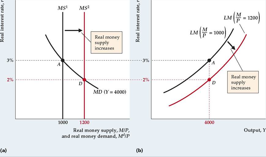
FIGURE 9.5
An increase in the real money supply shifts the LM curve down and to the right
(a) An increase in the real supply of money shifts the money supply curve to the right, from MS1 to MS2. For a constant level of output, the real interest rate that clears the asset market falls. If output is fixed at 4000, for example, the money demand curve is MD (Y = 4000) and the real interest rate that clears the asset market falls from 3% (point A) to 2% (point D).
(b) The graph shows the effect of the increase in real money supply on the LM curve. For any level of output, the increase in the real money supply causes the real interest rate that clears the asset market to fall. So, for example, when output is 4000, the increase in the real money supply causes the real interest rate that clears the asset market to fall from 3% (point A) to 2% (point D). Thus the LM curve shifts down and to the right, from LM (M/P = 1000) to LM (M∣P = 1200).
point A with a market-clearing real interest rate of 3%. The LM curve corresponding to the real money supply of 1000 is shown as LM (M/P = 1000) in Fig. 9.5(b). At point A on this LM curve, as at point A in the money supply-money demand diagram in Fig. 9.5(a), output is 4000 and the real interest rate is 3%. Because A lies on the initial LM curve, when output is 4000 and the money supply is 1000, the real interest rate that clears the asset market is 3%.
Now suppose that, with output constant at 4000, the real money supply rises from 1000 to 1200. This increase in the real money supply causes the vertical money supply curve to shift to the right, from MS1 to MS2 in Fig. 9.5(a). The asset market equilibrium point is now point D, where, with output remaining at 4000, the marketclearing real interest rate has fallen to 2%.
Why has the real interest rate that clears the asset market fallen? At the initial real interest rate of 3%, there is an excess supply of money—that is, holders of wealth have more money in their portfolios than they want to hold and, consequently, they have a smaller share of their wealth than they would like in nonmonetary assets. To eliminate this imbalance in their portfolios, holders of wealth will want to use some of their money to buy nonmonetary assets. However, when holders of wealth as a group try to purchase nonmonetary assets, the price of nonmonetary assets is bid up and hence the real interest rate paid on these assets declines. As the real interest rate falls, nonmonetary assets become less attractive relative to money. The real interest rate continues to fall until it reaches 2% at point D in Fig. 9.5(a), where the excess supply of money and the excess demand for nonmonetary assets are eliminated and the asset market is back in equilibrium.
The effect of the increase in the real money supply on the LM curve is illustrated in Fig. 9.5(b). With output constant at 4000, the increase in the real money supply lowers the real interest rate that clears the asset market, from 3% to 2%. Thus point D, where Y = 4000 and r = 2%, is now a point of asset market equilibrium, and point A no longer is. More generally, for any level of output, an increase in the real money supply lowers the real interest rate that clears the asset market. Therefore the entire LM curve shifts down and to the right. The new LM curve, for M/P = 1200, passes through the new equilibrium point D and lies below the old LM curve, for M/P = 1000.
Thus with fixed output, an increase in the real money supply lowers the real interest rate that clears the asset market and causes the LM curve to shift down and to the right. A similar analysis would show that a drop in the real money supply causes the LM curve to shift up and to the left.
What might cause the real money supply to increase? In general, because the real money supply equals M∣P, it will increase whenever the nominal money supply, M, which is controlled by the central bank, increases proportionately more than the price level increases.
Changes in Real Money Demand. A change in any variable that affects real money demand, other than output or the real interest rate, will also shift the LM curve. More specifically, with output constant, an increase in real money demand raises the real interest rate that clears the asset market and thus shifts the LM curve up and to the left. Analogously, with output constant, a drop in real money demand shifts the LM curve down and to the right.
Figure 9.6 shows a graphical analysis of an increase in money demand similar to that for a change in money supply shown in Fig. 9.5. As before, the money supplymoney demand diagram is shown on the left, Fig. 9.6(a). Output is constant at 4000, and the real money supply again is 1000. The initial money demand curve is MD1. The initial asset market equilibrium point is at A, where the money demand curve, MD1, and the money supply curve, MS, intersect. At initial equilibrium, point A, the real interest rate that clears the asset market is 3%.
Now suppose that, for a fixed level of output, a change occurs in the economy that increases real money demand. For example, if banks decided to increase the interest rate paid on money, im, the public would want to hold more money at the same levels of output and the real interest rate. Graphically, the increase in money demand shifts the money demand curve to the right, from MD1 to MD2 in Fig. 9.6(a). At the initial real interest rate of 3%, the real quantity of money demanded is 1300, which exceeds the available supply of 1000; so 3% is no longer the value of the real interest rate that clears the asset market.
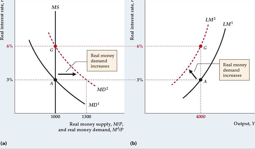
FIGURE 9.6
An increase in real money demand shifts the LM curve up and to the left
(a) With output constant at 4000 and the real money supply at 1000, an increase in the interest rate paid on money raises real money demand. The money demand curve shifts to the right, from MD1 to MD 2, and the real interest rate that clears the asset market rises from 3% (point A) to 6% (point G).
(b) The graph shows the effect of the increase in real money demand on the LM curve. When output is 4000, the increase in real money demand raises the real interest rate that clears the asset market from 3% (point A) to 6% (point G). More generally, for any level of output, the increase in real money demand raises the real interest rate that clears the asset market. Thus the LM curve shifts up and to the left, from LM1 to LM 2.
How will the real interest rate that clears the asset market change after the increase in money demand? If holders of wealth want to hold more money, they will exchange nonmonetary assets for money. Increased sales of nonmonetary assets will drive down their price and thus raise the real interest rate that they pay. The real interest rate will rise, reducing the attractiveness of holding money, until the public is satisfied to hold the available real money supply (1000). The real interest rate rises from its initial value of 3% at A to 6% at G.
Figure 9.6(b) shows the effect of the increase in money demand on the LM curve. The initial LM curve, LM1, passes through point A, showing that when output is 4000, the real interest rate that clears the asset market is 3%. (Point A in Fig. 9.6b corresponds to point A in Fig. 9.6a.) Following the increase in money demand, with output fixed at 4000, the market-clearing real interest rate rises to 6%. Thus the new LM curve must pass through point G (corresponding to point G in Fig. 9.6a), where Y = 4000 and r = 6%. The new LM curve, LM2, is higher than LM1 because the real interest rate that clears the asset market is now higher for any level of output.
9.4