The /S Curve: Equilibrium in the Goods Market
Discuss factors that affect the IS curve, which represents equilibrium in the goods market.
The second of the three markets in our model is the goods market. Recall from Chapter 4 that the goods market is in equilibrium when desired investment and desired national saving are equal or, equivalently, when the aggregate quantity of goods supplied equals the aggregate quantity of goods demanded.
Recall that adjustments in the real interest rate help bring about equilibrium in the goods market.In a diagram with the real interest rate on the vertical axis and real output on the horizontal axis, equilibrium in the goods market is described by a curve called the IS curve. For any level of output (or income), Y, the IS curve shows the real interest rate, r, for which the goods market is in equilibrium. The IS curve is so named because at all points on the curve desired investment, Id, equals desired national saving, Sd.
Figure 9.2 shows the derivation of the IS curve from the saving-investment diagram introduced in Chapter 4 (see Key Diagram 3). Figure 9.2(a) shows the saving-investment diagram drawn for two arbitrarily chosen levels of output, 4000 and 5000. Corresponding to each level is a saving curve, with the value of output indicated in parentheses next to it. Each saving curve slopes upward because an increase in the real interest rate causes households to increase their desired level of saving. An increase in current output (income) leads to more desired saving at any real interest rate, so the saving (S) curve for Y = 5000 lies to the right of the saving (S) curve for Y = 4000.
Also shown in Fig. 9.2(a) is an investment curve. Recall from Chapter 4 that the investment curve slopes downward. It slopes downward because an increase in the real interest rate increases the user cost of capital, which reduces the desired capital stock and hence desired investment.
Desired investment isn't affected by current output, so the investment curve is the same whether Y = 4000 or Y = 5000.Each level of output implies a different market-clearing real interest rate. When output is 4000, goods market equilibrium is at point D and the marketclearing real interest rate is 7%. When output is 5000, goods market equilibrium occurs at point F and the market-clearing real interest rate is 5%.
Figure 9.2(b) shows the IS curve for this economy, with output on the horizontal axis and the real interest rate on the vertical axis. For any level of output, the IS curve shows the real interest rate that clears the goods market. Thus Y = 4000 and r = 7% at point D on the IS curve. (Note that point D in Fig. 9.2b corresponds to point D in Fig. 9.2a.) Similarly, when output is 5000, the real interest rate that clears the goods market is 5%. This combination of output and the real interest rate occurs at point F on the IS curve in Fig. 9.2(b), which corresponds to point F in Fig. 9.2(a). In general, because a rise in output increases desired national saving, thereby reducing the real interest rate that clears the goods market, the IS curve slopes downward.
The slope of the IS curve may also be interpreted in terms of the alternative (but equivalent) version of the goods market equilibrium condition, which states that in equilibrium the aggregate quantity of goods demanded must equal the aggregate quantity of goods supplied. To illustrate, let's suppose that the economy is initially at point F in Fig. 9.2(b). The aggregate quantities of goods supplied and
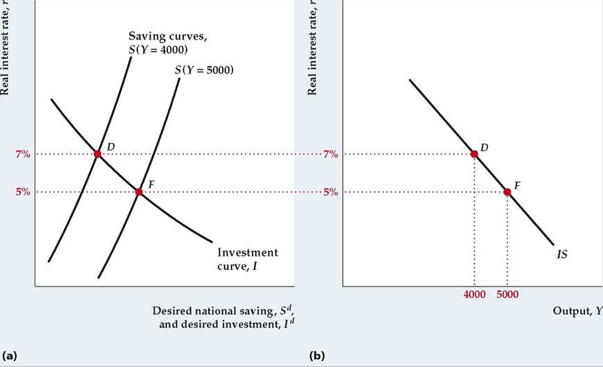
FIGURE 9.2
Deriving the /S curve
(a) The graph shows the goods market equilibrium for two different levels of output: 4000 and 5000 (the output corresponding to each saving curve is indicated in parentheses next to the curve). Higher levels of output (income) increase desired national saving and shift the saving curve to the right.
When output is 4000, the real interest rate that clears the goods market is 7% (point D). When output is 5000, the market-clearing real interest rate is 5% (point F).(b) For each level of output the IS curve shows the corresponding real interest rate that clears the goods market. Thus each point on the IS curve corresponds to an equilibrium point in the goods market. As in (a), when output is 4000, the real interest rate that clears the goods market is 7% (point D); when output is 5000, the market-clearing real interest rate is 5% (point F). Because higher output raises saving and leads to a lower market-clearing real interest rate, the IS curve slopes downward.
demanded are equal at point F because F lies on the IS curve, which means that the goods market is in equilibrium at that point.3
Now suppose that for some reason the real interest rate r rises from 5% to 7%. Recall from Chapter 4 that an increase in the real interest rate reduces both desired consumption, Cd (because people desire to save more when the real interest rate rises), and desired investment, Id, thereby reducing the aggregate quantity of goods demanded. If output, Y, remained at its initial level of 5000, the increase in the real interest rate would imply that more goods were being supplied than demanded. For the goods market to reach equilibrium at the higher real interest rate, the quantity of goods supplied has to fall. At point D in Fig. 9.2(b), output
3We have just shown that desired national saving equals desired investment at point F, or Sd = Id. Substituting the definition of desired national saving, Y — Cd — G, for Sd in the condition that desired national saving equals desired investment shows also that Y = Cd + Id + G at F.
has fallen enough (from 5000 to 4000) that the quantities of goods supplied and demanded are equal, and the goods market has returned to equilibrium.[151] Again, higher real interest rates are associated with less output in goods market equilibrium, so the IS curve slopes downward.
Factors That Shift the /S Curve
For any level of output, the IS curve shows the real interest rate needed to clear the goods market. With output held constant, any economic disturbance or policy change that changes the value of the goods-market-clearing real interest rate will cause the IS curve to shift. More specifically, for constant output, any change in the economy that reduces desired national saving relative to desired investment will increase the real interest rate that clears the goods market and thus shift the IS curve up and to the right. Similarly, for constant output, changes that increase desired saving relative to desired investment, thereby reducing the market-clearing real interest rate, shift the IS curve down and to the left. Factors that shift the IS curve are described in Summary table 12.
| SUMMARY 12 | ||
| Factors That Shift the /S | Curve | |
| An increase in | Shifts the /S curve | Reason |
| Expected future output | Up and to the right | Desired saving falls (desired consumption rises), raising the real interest rate that clears the goods market. |
| Wealth | Up and to the right | Desired saving falls (desired consumption rises), raising the real interest rate that clears the goods market. |
| Government purchases, G | Up and to the right | Desired saving falls (demand for goods rises), raising the real interest rate that clears the goods market. |
| Taxes, T | No change or down and to the left | No change, if consumers take into account an offsetting future tax cut and do not change consumption (Ricardian equivalence); down and to the left, if consumers don't take into account a future tax cut and reduce desired consumption, increasing desired national saving and lowering the real interest rate that clears the goods market. |
| Expected future TFP | Up and to the right | Desired investment and desired consumption increase, raising the real interest rate that clears the goods market. |
| Effective tax rate on capital | Down and to the left | Desired investment falls, lowering the real interest rate that clears the goods market. |
We can use a change in current government purchases to illustrate IS curve shifts in general.
The effects of a temporary increase in government purchases on the IS curve are shown in Figure 9.3. Figure 9.3(a) shows the saving-investment diagram, with an initial saving curve, S1, and an initial investment curve, I. The S1 curve represents saving when output (income) is fixed at Y = 4500. Figure 9.3(b) shows the initial IS curve, IS1. The initial goods market equilibrium when output, Y, equals 4500 is represented by point E in both (a) and (b). At E, the initial marketclearing real interest rate is 6%.Now suppose that the government increases its current purchases of goods, G. Desired investment at any level of the real interest rate isn't affected by the increase in government purchases, so the investment curve doesn't shift. However, as discussed in Chapter 4, a temporary increase in government purchases reduces desired national saving, Y — Cd — G (see Summary table 5 in Chapter 4), so the saving curve shifts to the left from S1 to S2 in Fig. 9.3(a). As a result of the reduction in desired national saving, the real interest rate that clears the goods market when output equals 4500 increases from 6% to 7% (point F in Fig. 9.3a).
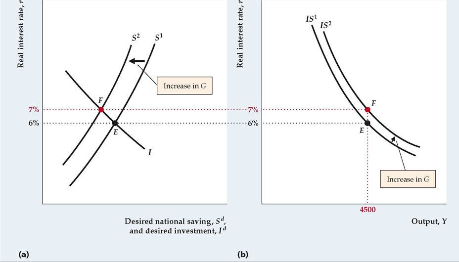
FIGURE 9.3
Effect on the /S curve of a temporary increase in government purchases
(a) The saving-investment diagram shows the effects of a temporary increase in government purchases, G, with output, Y, constant at 4500. The increase in G reduces desired national saving and shifts the saving curve to the left, from S1 to S2. The goods market equilibrium point moves from point E to point F, and the real interest rate rises from 6% to 7%.
(b) The increase in G raises the real interest rate that clears the goods market for any level of output. Thus the IS curve shifts up and to the right from IS1 to IS2. In this example, with output held constant at 4500, an increase in government purchases raises the real interest rate that clears the goods market from 6% (point E) to 7% (point F).
The effect on the IS curve is shown in Fig. 9.3(b). With output constant at 4500, the real interest rate that clears the goods market increases from 6% to 7%, as shown by the shift from point E to point F. The new IS curve, IS 2, passes through F and lies above and to the right of the initial IS curve, IS1. Thus a temporary increase in government purchases shifts the IS curve up and to the right.
So far our discussion of IS curve shifts has focused on the goods market equilibrium condition that desired national saving must equal desired investment. However, factors that shift the IS curve may also be described in terms of the alternative (but equivalent) goods market equilibrium condition—that the aggregate quantities of goods demanded and supplied are equal. In particular, for a given level of output, any change that increases the aggregate demand for goods shifts the IS curve up and to the right.
This rule works because, for the initial level of output, an increase in the aggregate demand for goods causes the quantity of goods demanded to exceed the quantity supplied. Goods market equilibrium can be restored at the same level of output by an increase in the real interest rate, which reduces desired consumption, Cd, and desired investment, Id. For any level of output, an increase in aggregate demand for goods raises the real interest rate that clears the goods market, so we conclude that an increase in the aggregate demand for goods shifts the IS curve up and to the right.
To illustrate this alternative way of thinking about shifts in the IS curve, we again use the example of a temporary increase in government purchases. Note that an increase in government purchases, G, directly raises the demand for goods, Cd + Id + G, leading to an excess demand for goods at the initial level of output. The excess demand for goods can be eliminated and goods market equilibrium at the initial level of output restored by an increase in the real interest rate, which reduces Cd and Id. Because a higher real interest rate is required for goods market equilibrium when government purchases increase, an increase in G causes the IS curve to shift up and to the right.
9.3