Agricultural Productivity and Industrialization

Although the models presented in the last two sections have highlighted how demand-side and supply-side factors can lead to structural change (and also how structural change can be consistent with a constant balanced growth path and the Kaldor facts), they did not focus on the process of industrialization.

the picture presented in Chapter 1, this question might hold important clues about the cross­country differences in income per capita today.

In this light, it would be useful to have a number of different approaches to this question and evaluate their pros and cons. Although this is part of my objective, I will not present these models all in one place. The first approach, based on the model of Acemoglu and Zilibotti (1997), was already presented as an application of stochastic growth models in Section 17.6 in Chapter 17. Although this theory focused on takeoff in general, the most relevant incident of takeoff in history is related to industrialization. Therefore, the theory in Section 17.6 can be interpreted as offering a potential explanation for the origins of industrialization based on whether the investments in different sectors undertaken by different societies turned out to be successful. In particular, societies that happen to have put a substantial fraction of their resources in sectors that turned out to be unlucky, or were ex post discovered not to be as productive, have been less successful than those that have invested in sectors and projects that were ex post more successful. The theory showed how success breeds success and a string of good outcomes can lead to a takeoff, whereby the society is able to diversify its sectoral and project-based risks successfully in a deeper financial markets and allocate its funds more productively towards high-return activities.

Before turning to market failures in development, it is useful to consider another ap­proach which will shed light on what factors might facilitate or even spur industrialization. A common argument in the economic history literature is that 18th-century England was par­ticularly well-placed for industrialization because of its high agricultural productivity (e.g., Nurske, 1953, Rostow, 1960, Mokyr, 1989, or Overton, 2001). The basic idea is that societies with a high agricultural productivity can afford to shift part of their labor force to indus­trial activities. Some type of increasing returns coming from technology or demand is then invoked to argue that the ability to shift a critical fraction of the labor force to industry is an important element of the early industrial experience.

In this section, I present a model based on Matsuyama (1992), which formalizes this intuition and presents a number of comparative static results that are useful in thinking about the origins of industrialization. Matsuyama’s model naturally complements the models

we have already studied in this chapter, because it is, at some level, a model of structural change. It combines Engel’s law and learning-by-doing externalities in the industrial sector.

Consider the following infinite-horizon continuous time economy with a constant popu­lation normalized to 1. The preference side is modeled via a representative household with preferences given by

which is similar to the preferences in (20.2). In particular, c^A (t) denotes the consumption of the agricultural good and c^M (t) is the consumption of the manufacturing good at time t. The parameter γA is again the minimum (subsistence) food requirement, ρ is the discount factor, and η designates the importance of agricultural goods versus manufacturing goods in the utility function. The representative household supplies labor inelastically. Let us also focus on the closed economy in the text, leaving some of the interesting extensions to open economy to Exercise 20.20.

Output in the two sectors is produced with the following production functions

and

where as before Y^m and Ya denote the total production of the manufacturing and the agricultural goods, and L^m and La denote the total labor employed in the two sectors. Both production functions F and G exhibit diminishing returns to labor. More formally, F and G are continuously differentiable and strictly concave. In particular, F(0) = 0, F⁰ (∙) > 0, F" (∙) < 0, G(0) = 0, G⁰ (∙) > 0, and G⁰⁰ (∙) < 0, where as usual F⁰ and G⁰ denotes first derivatives of these functions.

The key feature for this model of industrialization is that there is no technological progress in agriculture but the production function for the manufacturing good, (20.72), includes the term X (t), which will allow for technological progress in manufacturing. Although there is no technological progress in agriculture, the productivity parameter BA potentially differs across 837

countries, reflecting either previous technological progress in terms of new agricultural meth­ods or differences in land quality (even though here, for simplicity, we are focusing on a single country). Existing evidence shows that there are very large (perhaps too large) differences in labor productivity and TFP of agricultural activities among countries even today, thus allow­ing for potential productivity differences in agriculture is reasonable. Current research also shows that the image of the agricultural sector as a quasi-stagnant sector without technologi­cal progress is not accurate, and in fact, this sector experiences both substantial capital-labor substitution and major technological change (including the introduction of new varieties of seeds, mechanization, and organizational changes affecting productivity). Nevertheless, the current model provides a good starting point for our purposes.

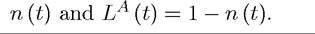
Labor market clearing requires that

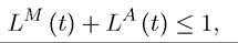
since total the labor supply is normalized to 1. Let n (t) denote the fraction of labor employed in manufacturing as of time t. Since there will be full employment in this economy, L^m (t) =

The key assumption is that manufacturing productivity, X (t), evolves over time as a result of learning-by-doing externalities as in Romer’s (1986) model we studied in Chapter 11.

where δ > 0 measures the extent of these learning-by-doing effects and we have an initial productivity level of X (0) > 0 at time t = 0 taken as given. As in the Romer model, learning-by-doing effects are external to individual firms. This type of external learning-by- doing effects are too reduced-form to generate insights about how productivity improvements take place in the industrial sector. Nevertheless, our analysis so far makes it clear that one can endogenize technology choices by introducing monopolistic competition and under the standard assumptions made in Part 4 above, this will generate a market size affect and lead to an equation similar to (20.74). Exercise 20.19 asks you to consider such a model.

In equilibrium, each firm will choose its labor demand in order to equate the value of the marginal product to the wage rate, w (t). Let us choose the price of agricultural goods as the numeraire (i.e., normalize it to 1) and also assume that the equilibrium is interior with both sectors being active. Then, equilibrium labor demand equations in the two sectors will be given by

where p (t) is the relative price of the manufactured good (in terms of the numeraire, the agricultural good). Market clearing then implies:

838

The presence of the term γA > 0 implies that as in Section 20.1, preferences are non- homothetic and that the income elasticity of demand for agricultural goods will be less than unity (while that for manufacturing goods will be greater than unity). As we have already seen, this is the simplest way of introducing Engel’s law.

Let us also assume that aggregate productivity is high enough to meet the minimum agricultural consumption requirements of the entire population (which, here, is normalized to 1):

If this inequality were violated, the economy’s agricultural sector would not be productive enough to provide the subsistence level of food to all consumers.

Finally, the budget constraint of the representative household at each date t can be written as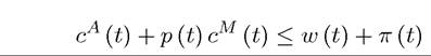

where π (t) is the profits per representative household, resulting from the diminishing returns in the production technologies.

An equilibrium in this economy is defined in the standard way as a sequence of consump­tion levels in the two sectors and allocations of labor between the two sectors at all dates, such that consumers maximize utility and firms maximize profits given prices, and goods and factor prices are such that all markets clear.

Maximization of (20.71) implies that for each household, and thus for the entire economy, we have

Since the economy is closed, production must equal consumption and thus

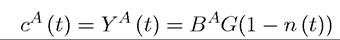
and

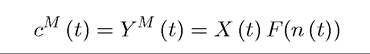
Now combining these equations with (20.75) and (20.77) yields

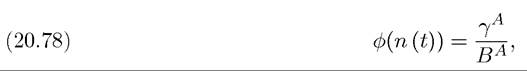
where

839

is a strictly decreasing function. Moreover, we have that φ(0) = G(1) and φ(1) < 0. The φ function can be interpreted as the “excess demand” function for manufacturing over agricul­ture. An equilibrium has to satisfy (20.78). From Assumption (20.76) and the properties of the φ function, we can conclude that the equilibrium condition (20.78) has a unique interior solution in which

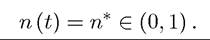
Notice an important implication of this equation. Even though the current model is one of structural change like those in the previous two sections, it only generates changes in the composition of output—the fraction of the labor force working in agriculture remains constant at 1 — n*. This implies that, while the current model is useful for interpreting the origins of industrialization, it will not be sufficient to generate insights about why the composition of employment in different sectors of the economy has been changing over the past 150 or 200 years.

Next, using (20.78), the unique equilibrium allocation of labor between the two sectors satisfies

(20.79)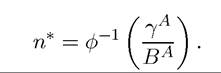

Since φ is strictly decreasing, so is its inverse function φ^-1 and thus the fraction of the labor force employed in manufacturing, n*, is strictly increasing in BA. This is the most important result of the current model and shows that a greater fraction of the labor force will be allocated to the manufacturing sector when agricultural productivity is higher. The reason for this result is intuitive: the Cobb-Douglas production function combined with homothetic preferences would imply a constant allocation of employment between the two sectors independent of their productivity. However, in the current model, preferences are non-homothetic preferences and a certain amount of food production is necessary first. When agricultural productivity, BA, is high, a relatively small fraction of the labor force is sufficient to generate this minimal level of food production, and thus a greater fraction of the labor force can be employed in manufacturing.

This results, combined with learning-by-doing in manufacturing, cf. equation (20.74), is at the root of the relationship between agricultural productivity and industrialization. In particular, equation (20.74) implies that output in manufacturing grows at the constant rate, δF(n*), which is also positively related to BA in view (20.79). Therefore, the current model generates a very simple representation of the often-hypothesized relationship between agricultural productivity and the origins of industrialization.

It is also useful to note that in the equilibrium of this model, because the shares of em­ployment in manufacturing and agriculture are constant and there is no technological progress in the agricultural sector, agricultural output remains constant. All growth is generated by 840

growth of manufacturing production. However, since manufacturing and agricultural goods are imperfect substitutes, the relative prices change, so expenditure on agricultural goods increases (see Exercise 20.18).

We can summarize these results as follows:

Proposition 20.12. In the above-described model, the combination of learning-by-doing and Engel's law generates a unique equilibrium in which the share of employment of manu­facturing is constant at n* ? φ^-1(γA/BA), and manufacturing output and consumption grow at the rate δF (n*), which is increasing in agricultural productivity BA.

We have so far characterized the equilibrium in a closed economy. A major result of this model is that higher agricultural productivity leads to faster industrial growth and thus to faster overall growth. The reason for this is intuitive: higher agricultural productivity en­ables the economy to allocate a larger fraction of its labor force to the knowledge-producing sector, which is manufacturing (where knowledge-production is introduced in a reduced-form manner as in Romer’s (1986) model). Even though the presumption that most important knowledge-producing activities take place in the manufacturing sector is no longer generally accepted, this model provides a useful framework for the analysis of the origins of industri­alization. An important advantage of the current model is its tractability. This enables us to adapt it easily to analyze other related questions, such as the impact of trade opening on industrialization. This is done in Exercise 20.20. The striking result in this case is that the implications of the closed and the open economies are very different. For example, that ex­ercise shows that higher agricultural productivity, in the presence of international trade, can lead to delayed industrialization or even to deindustrialization, rather than being the source of rapid industrialization as in the closed economy. The reason for this is related to the forces we analyzed in Section 19.7 of Chapter 19; specialization according to comparative advan­tage may have negative long-run consequences in the presence of sector-specific externalities. However, as already discussed in that section, the evidence for large externalities of this sort are not very strong. Consequently, the model in this section and its implications regarding the role of international trade in the process of industrialization should be interpreted with some caution. Nevertheless, this model is an important tool in our arsenal of models of long-run economic development, especially because it illustrates in an elegant and tractable manner how agricultural productivity interacts with the process of industrialization.

20.3.