Non-Balanced Growth: The Supply Side

The previous section showed how the process of structural change can be driven by a generalized form of Engel’s law, that is, by the desires of the consumers to change the composition of their consumption as they become richer.

factors. Nevertheless, isolating these factors in separate models is both more tractable and also conceptually more transparent. For this reason, in this section I focus on the supply side, abstracting from Engel’s law throughout, and will only return to the combination of the supply-side and the demand-side factors in Exercise 20.17.

20.2.1. General Insights. At some level, Baumol’s theory of non-balanced growth can be viewed as self-evident—if some sectors have higher rates of technological progress, there must be some non-balanced elements in equilibrium. My first purpose in this section is to show that there are more subtle and compelling reasons for supply-side non-balanced growth than those originally emphasized by Baumol.

I will illustrate this point first using a simple but fairly general environment. This en­vironment consists of two sectors each with a constant returns to scale production function and arbitrary preferences over the goods that are produced in these two sectors. Both sectors employ capital, K, and labor, L. To highlight that the exact nature of the accumulation process is not essential for the results, I take the sequence (process) of capital and labor supplies,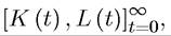as given and assume that labor is supplied inelastically.

Preferences are defined over the final output or a consumption aggregator as in (20.3) in the previous section. Whether we use the specification with a consumption aggregator or a formulation with intermediates used competitively in the production of a final good makes no difference for any of the results. With this in mind, let final output be denoted by Y and assume that it is produced as an aggregate of the output of two sectors, Yi and Y₂,

Let us also assume that F satisfies Assumptions 1 and 2, so that, in particular, it exhibits con­stant returns to scale and is twice continuously differentiable.

822

where L_i (t), Lq (t), K_i (t) and Kq (t) denote the amount of labor and capital employed in the two sectors, and the functions G_i and Gq are also assumed to satisfy the equivalents of Assumptions 1 and 2. The terms Ai (t) and Aq (t) are Hicks-neutral technology terms.

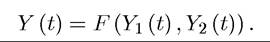
Market clearing for capital and labor implies that

at each t. Without loss of any generality, I ignore capital depreciation.

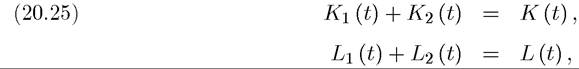
Let us take the final good as the numeraire in every period and denote the prices of Yi and Y2 by p∣ and p2, and wage and rental rate of capital (interest rate) by w and r. Product and factor markets are competitive, so that product and factor prices satisfy 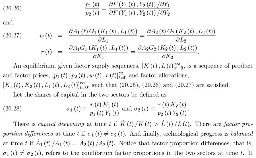does not necessarily mean that these will not be equal at some future date. The following proposition shows the supply side forces leading to structural change in the simplest possible way:

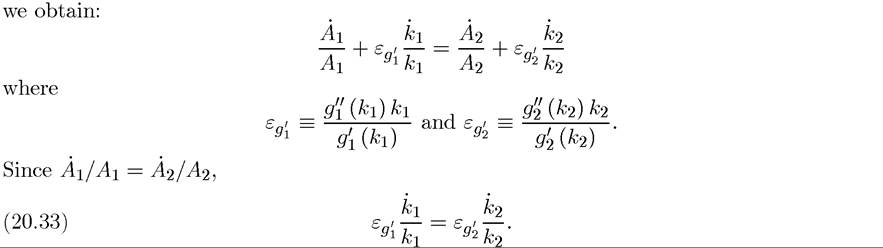
Proposition 20.5. Suppose that at time t, there are factor proportion differences between the two sectors, technological progress is balanced, and there is capital deepening, then growth

823

and the “per capita production functions” (without the Hicks-neutral technology term) as

Since Gi and G∙₂ are twice continuously differentiable by assumption, so are g₁ and g₂ and denote their first and second derivatives by

Now, differentiating the production functions for the two sectors,

Given the definition in (20.29), equation (20.27) gives the following conditions character­izing the equilibrium interest rate and wage:

and

Differentiating the interest rate condition, (20.31), with respect to time and using (20.30),

Differentiating the wage condition, (20.32), with respect to time, using (20.30) and some

Since A1/A1 = A2/A2 and σ1 = σ2, this equation is inconsistent with (20.33), yielding a contradiction and proving the claim.

The intuition for this result is straightforward. Suppose that there is capital deepening and that, for concreteness, sector 2 is more capital-intensive (i.e., σι < σ2). Now, if both capital and labor were allocated to the two sectors at constant proportions over time, the more capital-intensive sector, sector 2, would grow faster than sector 1. In equilibrium, the faster growth in sector 2 would change equilibrium prices, and the decline in the relative price of sector 2 would cause some of the labor and capital to be reallocated to sector 1. However, this reallocation could not entirely offset the greater increase in the output of sector 2, since, if it did, the relative price change that stimulated the reallocation would not take place. Consequently, equilibrium growth must be non-balanced.

Proposition 20.5 is related to the well-known Rybczynski’s Theorem in international trade. Rybczynski’s Theorem states that for an open economy within the “cone of diver­sification” (where factor prices do not depend on factor endowments), changes in factor endowments will be absorbed by changes in the sectoral output mix. Proposition 20.5 can be viewed both as a closed-economy analog and also as a generalization of Rybczynski’s The­orem; it shows that changes in factor endowments (capital deepening) will be absorbed by faster growth in one sector than the other, even though relative prices of goods and factors will change in response to the change in factor endowments.

It is also straightforward to generalize Proposition 20.5 to an economy with N ≥ 2 sectors. In particular, suppose that aggregate output is given by the constant returns to scale production function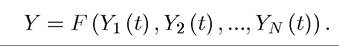

Defining σj (t) as the capital share in sector j = 1,...,N as in (20.28), we have:

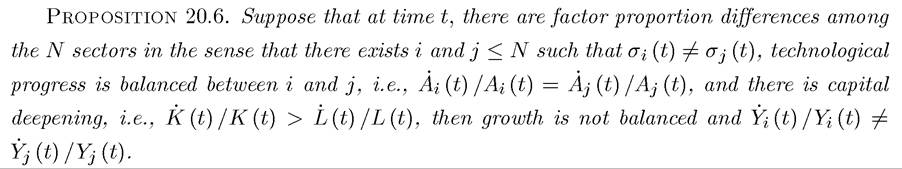
Proof.

20.2.2. Balanced Growth and Kuznets Facts. The previous subsection provided general insights about how supply-side factors can lead to non-balanced growth. To obtain a general result on the implications of capital deepening and factor proportion differences across sectors on non-balanced growth, Proposition 20.5 was stated for a given (arbitrary) sequence of capital and labor supplies,However, without endogenizing the

path of capital accumulation (and specifying the pattern of population growth) we cannot address whether a model relying on supply-side factors can also provide a useful framework for thinking about the Kaldor and the Kuznets facts.

For this purpose, I now specialize the environment of the previous subsection by incorpo­rating specific preferences and production functions and then provide a full characterization of a simpler economy. The economy is again in infinite horizon and population grows at the exogenous rate n > 0 according to (20.1). Let us also assume that the economy admits a representative consumer, with standard preferences given by (20.2), who also supplies labor inelastically. Proposition 20.5 emphasized the importance of capital deepening, which will now result from exogenous technological progress.

Instead of a general production function for the final good as in the previous subsection, I now assume that the unique final good is produced with a constant elasticity of substitution aggregator:

where ε ∈ [0, ∞) is the elasticity of substitution between the two intermediates and γ ∈ (0,1) determines the relative importance of the two goods in aggregate production. Let us ignore capital depreciation again and also assume that the final good is distributed between consumption and investment, i.e.,

where c (t) is consumption per capita.

The two intermediates Yi and Y% are produced competitively with aggregate production functions

Throughout, I impose that

which implies that sector 1 is less capital-intensive than sector 2. This is without loss of any generality, since in the case in which αι = α2, there are no supply-side effects and thus the issues I am concerned with in this section do not arise.

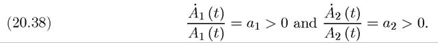
In (20.36) Ai and A∙₂ correspond to Hicks-neutral technology term that grow at exogenous and potentially different rates given by

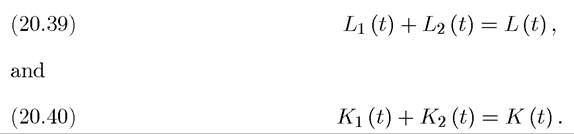
Labor and capital market clearing again require that at each t,

826

Let us also denote the wage and the interest rate (the rental rate of capital) by w (t) and r (t) and the prices of the two intermediate goods by pi (t) and ρ₂ (t). We again normalize the price of the final good to 1 at each instant. An equilibrium is defined in the usual manner, as se-

It is useful to break the characterization of equilibrium into two pieces: static and dy­namic. The static part takes the state variables of the economy, which are the capital stock, the labor supply and the technology, K, L, Ai and A2, as given and determines the allocation of capital and labor across sectors and the equilibrium factor and intermediate prices. The dynamic part of the equilibrium determines the evolution of the endogenous state variable, K (the dynamic behavior of L is given by (20.1) and those of Ai and A₂ by (20.38)).

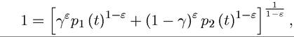
The choice of numeraire implies that at each instant

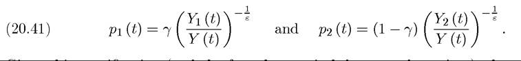
and profit maximization of the final good sector implies

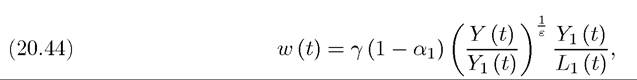
Given this specification (and the fact that capital does not depreciate), the equilibrium al­location of resources will equate the marginal product of capital and labor into two sectors. The following equations give these equilibrium conditions and also expressions for the factor prices (see Exercise 20.12). The equilibrium conditions are

while the factor prices can be expressed as

and

827

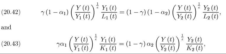
The key to the characterization of the static equilibrium is to determine the fraction of capital and labor employed in the two sectors. Let us define κ (t) ? K1 (t) /K (t) and λ (t) ? L₁ (t) /L (t). Combining equations (20.39), (20.40), (20.42), and (20.43), we obtain:

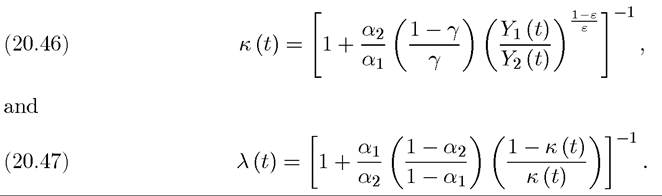
Equation (20.47) makes it clear that the share of labor in sector 1, λ, is monotonically increasing in the share of capital in sector 1, κ. This implies that in equilibrium capital and labor will be reallocated towards the same sector. The structure of the static equilibrium depends on how the allocation of capital and labor depends on the aggregate amount of capital and labor available in the economy. The following proposition answers this question.

Proposition 20.7. In equilibrium,

Proof. See Exercise 20.13.

Equation (20.48) states that when the elasticity of substitution between sectors, ε, is less than 1, the fraction of capital allocated to the capital-intensive sector declines in the stock of capital (and conversely, when ε > 1, this fraction is increasing in the stock of capital). Intuitively, if K increases and κ remains constant, then the capital-intensive sector, sector 2, will grow by more than sector 1. Equilibrium prices given in (20.41) then imply that when ε < 1 the relative price of the capital-intensive sector will fall more than proportionately, inducing a greater fraction of capital to be allocated to the less capital-intensive sector 1. The intuition for the converse result when ε > 1 is similar.

Moreover, equation (20.49) implies that when the elasticity of substitution, ε, is less than one, an improvement in the technology of a sector causes the share of capital going to that sector to fall. The intuition is again the same: when ε < 1, increased production in a sector causes a more than proportional decline in its relative price, inducing a reallocation of capital away from it towards the other sector (again the converse results and intuition apply when ε > 1).

Combining (20.44) and (20.45), we also obtain relative factor prices as

and the capital share in the economy as:

Proposition 20.8. In equilibrium,

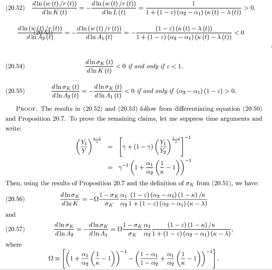
Clearly, Ω > 0 if and only if α⅛ < α2, which is satisfied in view of (20.37). Equations (20.56)

if and only if (α2 — αι)(1 — ε) > 0.

and (20.57) then imply (20.54) and (20.55).

The most important result in this proposition is (20.54), which links the equilibrium relationship between the capital share in national income and the capital stock to the elasticity of substitution. Since a negative relationship between the share of capital in national income and the capital stock is equivalent to capital and labor being gross complements in the aggregate, this result also implies that the elasticity of substitution between capital and labor is less than one if and only if ε is less than one. Recall from the discussion in Section 15.6 in Chapter 15 that a variety of different approaches suggest that the elasticity of substitution between capital and labor is less than one.

The intuition for Proposition 20.8 is informative about the workings of the model. Con­sistent with the discussion of Proposition 20.5 above, when ε < 1, an increase in the capital stock of the economy causes the output of the more capital-intensive sector, sector 2, to increase relative to the output in the less capital-intensive sector (despite the fact that the share of capital allocated to the less-capital intensive sector increases as shown in equation (20.48)). This then increases the production of the more capital-intensive sector and reduces the relative reward to capital (and the share of capital in national income). The converse result applies when ε > 1.

Recall also from Section 15.2 in Chapter 15 that when ε < 1, (20.55) in Proposition 20.8 implies that an increase in Ai is “capital biased” and an increase in A∙₂ is “labor biased”. The intuition for why an increase in the productivity of the sector that is intensive in capital is biased toward labor (and vice versa) is again similar: when the elasticity of substitution between the two sectors, ε, is less than one, an increase in the output of a sector (this time driven by a change in technology) decreases its price more than proportionately, thus reducing the relative compensation of the factor used more intensively in that sector. When ε > 1, we have the converse pattern, and an increase in A₂ is “capital biased,” while an increase in Ai is “labor biased”

We now turn to the characterization of the dynamic equilibrium path of this economy.

We start with the Euler equation for consumers, which follows from the maximization of

(20.2). The Euler equation for per capita consumption takes the familiar form:

Since the only asset of the representative household in this economy is capital, the transver- sality condition takes the standard form:

which, together with the Euler equation (20.58) and the resource constraint (20.35), deter­mines the dynamic behavior of consumption per capita and capital stock, c and K. Equations (20.1) and (20.38) give the behavior of L, Ai and A₂.

A dynamic equilibrium is given by paths of wages, interest rates, labor and capital alloca­tion decisions, w, r, λ and κ, satisfying (20.44), (20.42), (20.45), (20.43), (20.46) and (20.47), and of consumption per capita, c, capital stock, K, employment, L, and technology, Ai and A₂, satisfying (20.1), (20.35), (20.38), (20.58), and (20.59).

Let us also introduce the following notation for growth rates of the key ob jects in this

economy:

Whenever they exist, we can also define the corresponding (limiting) asymptotic growth rates

as follows:

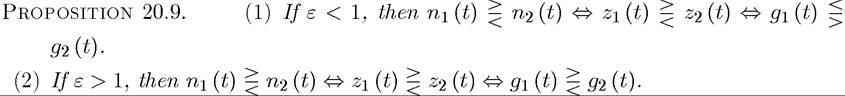
Proof. Omitting time arguments and differentiating (20.42) with respect to time, we obtain

which implies that ni - n2 = (ε - 1) (qi - q2) /ε and establishes the first part of the propo­

sition. Similarly differentiating (20.43) yields

and establishes the second part of the result.

?

This proposition establishes the straightforward, but at first counter-intuitive, result that, when the elasticity of substitution between the two sectors is less than one, the equilibrium growth rate of the capital stock and labor force in the sector that is growing faster must be less than in the other sector. When the elasticity of substitution is greater than one, the converse result obtains. To see the intuition, note that terms of trade (relative prices) shift in favor of the more slowly growing sector. When the elasticity of substitution is less than one, this change in relative prices is more than proportional with the change in quantities and this encourages more of the factors to be allocated towards the more slowly growing sector.

Proof. Differentiating the production function for the final good (20.34) we obtain:

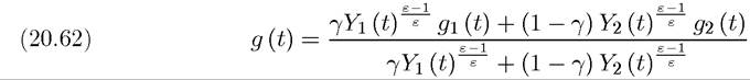
Consequently, when the elasticity of substitution is less than 1, the asymptotic growth rate of aggregate output will be determined by the sector that is growing more slowly, and the converse applies when ε > 1.

As in the previous section, we focus on a constant growth path (CGP), again defined as an equilibrium path where the asymptotic growth rate of consumption per capita exists and

Let us also define the growth rate of total consumption as C (t) /C (t) ? g*_c = g* + n, since it will be slightly more convenient to work with the growth rate of total consumption than the growth rate of consumption per capita. From the Euler equation (20.58), the fact that the growth rate of consumption or consumption per capita are asymptotically constant implies

that the interest rate must also be asymptotically constant, that is, lim_t→∞ r = 0.

To establish the existence of a CGP, we impose the following parameter restriction:

This assumption ensures that the transversality condition (20.59) holds. Terms of the form αι/(1 — αι) or a₂/ (1 — op) appear naturally in equilibrium, since they capture the “aug­mented” rate of technological progress. In particular, recall that associated with the tech-

nological progress, there will also be endogenous capital deepening in each sector. The overall effect on labor productivity (and output growth) will depend on the rate of techno­logical progress augmented with the rate of capital deepening. The terms αι/ (1 — αι) or a2/ (1 — «2) capture this, since a lower α_s corresponds to a greater share of capital in the sector s = 1, 2, and thus to a higher rate of augmented technological progress for a given rate of Hicks-neutral technological change. In this light, condition (20.63) can be understood as implying that the augmented rate of technological progress should be low enough to satisfy the transversality condition (20.59).

The next proposition will present the main result of this subsection and will characterize the relatively simple form of the CGP in the presence of non-balanced growth. However, rather than presenting the general case, it is useful to impose the following assumption (20.64)

832

which will make it easier to state this result. In particular, this condition ensures that sector 1 is the asymptotically dominant sector, either because it has a slower rate of technological progress and ε < 1, or it has more rapid technological progress and ε > 1. Notice also that, for the reasons noted above, the appropriate comparison is not between α∣ and a%, but between αι/ (1 — αι) and a%/ (1 — α2). Exercise 20.14 generalizes the results in this proposition to the case in which the converse of condition (20.64) holds.

Proposition 20.11. Suppose that conditions (20.37), (20.63) and (20.64) hold. Then there exists a unique CGP such that

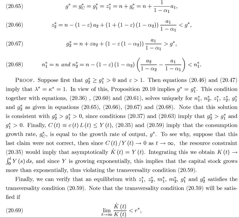
where r* is the constant asymptotic interest rate. Since from the Euler equation (20.58) r* = θg* + ρ, (20.69) will be satisfied when g² (1 — θ) < p. Condition (20.63) ensures that this is the case with g* = n + αι/ (1 — αι). The argument for the case in which g2 ≥ g2 > 0 and ε > 1 is similar and is left to Exercise 20.14.

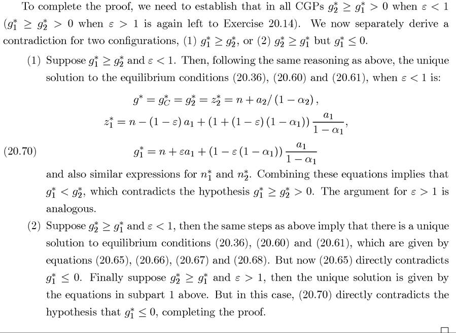
A number of implications of this proposition are worth emphasizing. First, as long as 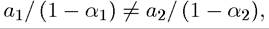growth is non-balanced. The intuition for this result is the same as Proposition 20.5 in the previous subsection. Suppose, for concreteness, that ai/ (1 — αq) < ^a2/ (1 — «2) (which would be the case, for example, if ai ≈ α2). Then, differential capital intensities in the two sectors combined with capital deepening in the economy (which itself results from technological progress) ensures faster growth in the more capital-intensive sector, sector 2. Intuitively, if capital were allocated proportionately to the two sectors, sector 2 would grow faster. Because of the changes in prices, capital and labor are reallocated in favor of the less capital-intensive sector, so that relative employment in sector 1 increases. However, crucially, this reallocation is not enough to fully offset the faster growth of real output in the more capital-intensive sector. This result also highlights that the assumption of balanced technological progress in Proposition 20.5 (which, in this context, corresponds to ai = α2) was not necessary for the result there, but we simply needed to rule out the knife-edge case where the relative rates of technological progress between the two sectors were exactly in the right proportion to ensure balanced growth (in this context, ai/ (1 — αq) = a2/ (1 — α₂)).

Second, the CGP growth rates are relatively simple, especially because we have restricted attention to the set of parameters that ensure that sector 1 is the asymptotically dominant 834

sector (cf., condition (20.64)). If, in addition, we also have ε < 1, the model leads to the richest set of dynamics, whereby the more slowly growing sector determines the long-run growth rate of the economy, while the more rapidly growing sector continually sheds capital and labor, but does so at exactly the right rate to ensure that it still grows faster than the rest of the economy.

Third, in the limiting equilibrium the share of capital and labor allocated to one of the sector tends to one (e.g., when sector 1 is the asymptotically dominant sector, λ* = κ* = 1). Nevertheless, at all points in time both sectors produce positive amounts, so this limit point is never reached. In fact, at all times both sectors grow at rates greater than the rate of population growth in the economy. Moreover, when ε < 1, the sector that is shrinking grows faster than the rest of the economy at all point in time, even asymptotically. Therefore, the rate at which capital and labor are allocated away from this sector is determined in equilibrium to be exactly such that this sector still grows faster than the rest of the economy. This is the sense in which non-balanced growth is not a trivial outcome in this economy (with one of the sectors shutting down), but results from the positive but differential growth of the two sectors.

Finally, it can be verified that the capital share in national income and the interest rate are constant in the CGP. For example, when condition (20.64) holds, we haveIn

contrast, when this condition does not holdin other words, the asymptotic capital

share in national income will reflect the capital share of the dominant sector. It can also be verified that limiting interest rate is also constant (see Exercise 20.15), thus this model based on supply-side sources of non-balanced growth is also consistent with the Kaldor facts as well as the Kuznets facts. The analysis so far does not establish that the CGP is asymptotically stable. This is done in Exercise 20.16, which also provides an alternative proof of Proposition

20.11. Consequently, a model based on supply-side factors can also give useful insights about structural change. Naturally, to understand a sweeping long-run changes in the composition of output and employment, we need to combine the demand-side and the supply-side factors studied in the last two sections. Exercise 20.17 takes a first step in this direction.

20.3.