Non-Balanced Growth: The Demand Side

Figure 20.1 provides a summary of some of the major changes in the structure of produc­tion that the US economy has undergone over the past 150 years. It shows that the share of US employment in agriculture stood at around 90% of the labor force at the beginning of the 19th century, while only a very small fraction of the US labor force worked in manufacturing and services.

agricultural goods). The changes in the composition of employment in the British economy towards the end of the 18th century are also consistent with the US patterns shown in Figure 20.1 (see, for example, Mokyr, 1989). Consequently, similar patterns are present in all OECD economies. Some of the less-developed economies are still largely agricultural but the time trend is inexorably towards a smaller share of agriculture. Because of Kuznets’s emphasis on structural change and seminal work on the topic, Kongsamut, Rebelo and Xie (2001) refer to these changes in the composition of employment and production as the Kuznets facts. They provide a tractable model to reconcile this type of structural change with the Kaldor facts we have emphasized so far, that is, the relative constancy of factor shares and the interest rate.

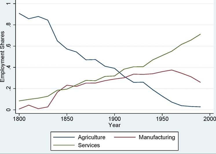
Figure 20.1. The share of US employment in agriculture, manufacturing and services, 1800-2000.

Figure 20.1 paints a picture of changes in sectoral employment that includes a signifi­cant non-balanced component. Consequently, models that depart from Kaldor facts over the early stages of the development process might be useful for understanding broader aspects of structural change. Kongsamut, Rebelo and Xie instead take a more modest departure from the baseline neoclassical growth model and propose a model that can account for a certain degree of non-balanced growth at the sectoral level, while still remaining consistent with the 814

Kaldor facts of aggregate balanced growth. Even though it is designed to match the Kaldor facts regardless of the stage of development, its tractability makes this model a useful start­ing point for our analysis. Moreover, as emphasized by Kuznets, once we look beneath the aggregate facts of balanced growth structural changes in the composition of employment and production are present even in relatively advanced economies. A model consistent with the Kaldor facts provides us with the simplest approach to these types of sectoral changes that appear to be ongoing even in relatively developed economies.

At the heart of Kongsamut, Rebelo and Xie’s approach is the so-called Engel's law, which states that as a household’s income increases, the fraction that it spends on food (agricultural products) declines. While calling this observation a law may exaggerate its status, this observation first made by the 19th-century German statistician Ernst Engel, appears to be a remarkably robust pattern in the data. Kongsamut, Rebelo and Xie extend Engel’s law, by also positing that as a household becomes richer, it will desire not only to spend less on food, but will also wish to spend more on services. In particular, consider the following infinite-horizon economy.

The economy admits a representative household who supplies labor inelastically and has standard preferences given by

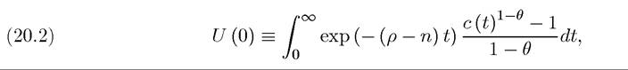
with θ ≥ 0 and c (t) denoting the consumption aggregate produced out of agricultural, man­ufacturing and service goods. I use the lower case letter here to emphasize that this is con­sumption per capita. Aggregate consumption itself consists of agricultural, manufacturing and services consumptions, with an aggregator of the form:

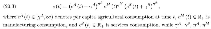
and η^s are positive constants. This general functional form of the aggregator (preferences) is often referred to as the Stone-Geary preferences. It is a highly tractable way of introducing income elasticities that are different from one for different subcomponents of consumption, which will enable us to incorporate Engel’s law. In particular, this aggregator implies that there is a minimum or subsistence level of agricultural (food) consumption equal tcThe

household must consume at least this much food to survive and in fact, consumption and utility are not defined when the household does not consume the minimum amount of food (recall (negative number)^1-θ is undefined for θ > 0). After this level of food consumption 815

has been achieved, the household starts to demand other items, in particular, manufactured goods (e.g., textiles and durables) and services (entertainment, retail, etc.). However, as we will see shortly, the presence of the γ^s term in the aggregator implies that the household will spend a positive amount on services only after certain levels of agricultural and manufacturing consumption have been reached.

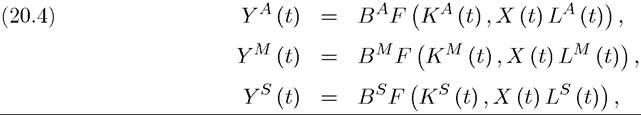
We assume that the economy is closed, thus agricultural, manufacturing and services consumption must be met by domestic production. We follow Kongsamut, Rebelo and Xie and assume the following production functions for the agricultural, manufacturing and service goods:

where idenotes the output of agricultural, manufacturing and services

at time t,are the levels of capital and labor allocated

to the agricultural, manufacturing and services sectors at time t,is a

Hicks-neutral productivity term for the three sectors and finally, X (t) is a labor-augmenting (Harrod-neutral) productivity term affecting all sectors (I use the letter X instead of the standard A to distinguish this from the agricultural good). The function F satisfies the usual neoclassical assumptions, Assumptions 1 and 2, and thus in particular, exhibits constant returns to scale. Two other features in (20.4) are worth noting. First, the production function for all three sectors are identical. Second, the same labor-augmenting technology term affects all three sectors. Both of these features are clearly unrealistic but they are useful to isolate the demand-side sources of structural change and to contrast them with the supply-side factors that will be discussed in the next section. Furthermore, Exercises 20.7 below show that they can be relaxed to some degree. Throughout we take the initial population, L (0) > 0, and the initial capital stock, K (0) > 0, as given. Let us also assume that there is a constant rate of growth of the labor-augmenting technology term, i.e.,

for all t, with initial condition X (0) > 0.

Market clearing for labor and capital requires

and

where K (t) and L (t) are the total supplies of capital and labor at time t.

Another key assumption of the Kongsamut, Rebelo and Xie model builds on Rebelo (1991) and imposes that it is the manufacturing good that is used in the production of the investment good. Consequently, market clearing for the manufacturing good takes the form where, for simplicity, we have ignored capital depreciation (otherwise there would be an additional term δK (t) on the left-hand side). This equation states that the total production of manufacturing goods is distributed between consumption of manufacturing goods and new capital stock, which will be used for production of agricultural, manufacturing and service goods in the future. Since the economy admits a representative household, equations (20.4)­(20.8) can also be taken to represent the representative household’s budget constraint.

In addition, market clearing for the agricultural and service goods take the standard forms

where the left-hand sides of both equations are multiplied by L (t) to turn per capita con­sumption levels into total consumptions.

All market are competitive. Let us choose the price of the manufacturing good at each date as the numeraire, which leaves us with the prices of agricultural goods, p^A (t), and of services, p^s (t), and factor prices w (t) and r (t).

and

Competitive factor markets also imply

and

where I could have equivalently used the marginal products from other sectors, with identical results.

A competitive equilibrium is defined in the usual manner as sequences of sectoral fac- so that the economy starts with enough capital and technological know-how to produce more than the minimum necessary amount of agricultural consumption

An equilibrium is straightforward to characterize in this economy. Because the production functions of the all three sectors are identical, the following result obtains immediately:

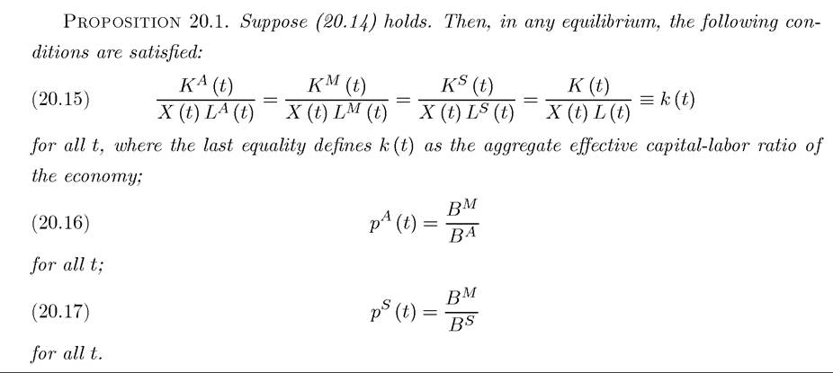
Proof. See Exercise 20.2.

?

The results in this proposition are intuitive. First, the fact that the production functions are identical implies that the capital-labor ratios allocated to the three sectors must be equalized. Second, given (20.15), the equilibrium price relationships (20.16) and (20.17) follow from the fact that the marginal products of capital and labor have to be equalized in all three sectors.

Proposition 20.1 does not make use of the preference side. Next incorporating utility maximization on the side of the representative household, in particular, deriving the standard Euler equation for the representative consumer and then using equations (20.10)-(20.11), we obtain the following additional equilibrium conditions:

Proposition 20.2. Suppose (20.14) holds. Then, in any equilibrium, we have that

(20.18)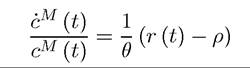

for all t and moreover, provided that Assumption 4 holds, the transversality condition of the representative household is satisfied. In addition, we have that for all t

and

Proof. See Exercise 20.3. ?

In analogy to previous models we have seen so far, we may want to define a balanced growth path in this economy as an equilibrium path in which output and consumption of all three sectors grow at the same constant rate. The next proposition shows that such a balanced growth path does not exist.

Proposition 20.3. Suppose that either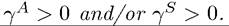Then a balanced growth

path does not exist.

Proof. See Exercise 20.4. ?

This result is not surprising. Since the preferences of the representative household in­corporate Engel’s law, the household would always like to change the composition of its consumption, and this will be reflected in a change in the composition of production. In­stead of a balanced growth path, let us define a weaker notion of “balanced growth,” which I will refer to as a constant growth path (CGP). A CGP requires that the rate of growth of aggregate consumption must be asymptotically constant.¹ Given the preferences in (20.2), the constant growth rate of consumption implies that the interest rate must also be constant asymptotically. In a CGP, output, consumption and employment in the three sectors may grow at different rates.

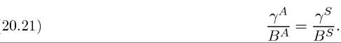
Proposition 20.4. Suppose (20.14) holds. Then, in the above-described economy a CGP exists if and only if

^[1]Kongsamut, Rebelo and Xie, instead, define the concept of generalized balanced growth path, where the interest rate is constant. Clearly, given the CRRA preferences in (20.2), the two notions are equivalent.

In a CGP k (t) = k* for all t, and moreover we have the following evolution of consumption

and employment in the three sectors

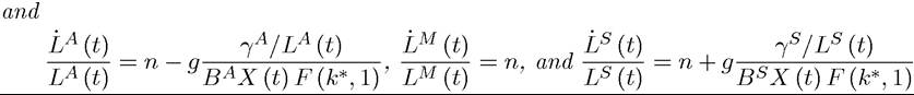
for all t.

Moreover, in the CGP the share of national income accruing to capital is constant.

Proof. See Exercise 20.5.

This model therefore delivers a tractable framework for the analysis of structural change that has potential relevance both for the experience of economies at the early stages of devel­opment and also for understanding the patterns of growth of relatively advanced countries. Engel’s law (augmented with the highly income elastic demand for services) generates a demand-side force towards non-balanced growth. In particular, as their incomes grow, con­sumers wish to spend a greater fraction of their budget on services and a smaller fraction on food (agricultural goods). This makes an equilibrium with fully balanced growth impossible. Instead, different sectors grow at different rates and there is reallocation of labor and capital across sectors. Nevertheless, Proposition 20.4 shows that under condition (20.21) a constant growth path (CGP) exists and in this equilibrium, structural change takes place despite the fact that the interest rate and the share of capital in national income are constant. This model therefore delivers many of the features that are useful for thinking of the long haul of the process of development; in particular, the equilibrium path can be consistent with the Kaldor facts, and there is a continuous process of structural change, whereby the share of agriculture in production and employment declines over the development process and the share of services increases.

On the downside, a number of potential shortcomings of the current model are worth noting. First, one may argue that the process of structural change in this model falls short of the sweeping transformations discussed by Kuznets. It is straightforward to incorporate transitional dynamics into the model. Exercise 20.6 shows that if the effective capital-labor ratio starts out below its CGP value of k* in Proposition 20.4, then there will be additional transitional dynamics in this model complementing the structural changes. Nevertheless, even these transitional dynamics probably fall short of the sweeping structural change emphasized by Kuznets. To some degree, whether or not this is so is a matter of taste and emphasis. The current model certainly does not incorporate the various different aspects of structural transformation which we will discuss in the next chapter, though it was also not meant to incorporate these transformations.

Second, the assumption that all three sectors have the same production function appears restrictive. Nevertheless, this assumption can be relaxed to some degree. Exercise 20.7 discusses how this can be done. Perhaps more important is the assumption that investments for all three sectors use only the manufacturing good. This assumption is similar in nature to the assumption that only capital is used to be produce capital (investment) goods in Rebelo’s (1991) model, which we studied in Chapter 11. Exercise 20.10 shows that if this assumption is relaxed, it is no longer possible to reconcile the Kuznets and the Kaldor facts in the context of this model.

Third, the model presented here is designed to generate a constant share of employment in manufacturing. Although this pattern is broadly consistent with the US experience over the past 150 years, when we look at even earlier stages of development, almost all employment is in agriculture. This implies that early stages of structural change must also involve an increase in the share of employment in manufacturing. A number of models in the literature generate this pattern by also introducing land as an additional factor of production. Exercise 20.8 provides an example and Section 21.2 will further discuss models incorporating land as a major factor of production in the context of the study of population dynamics.

Finally, the condition necessary for a CGP, (20.21), is a rather “knife-edge” condition. We would not expect this condition to be satisfied naturally. Nevertheless, even when this condition is not satisfied, the behavior of the model may approximate the structural change we observe in practice and Exercise 20.9 illustrates this with an example in which sectoral production functions differ but are all of the Cobb-Douglas form.

20.2.