Appendix 9.B Algebraic Versions of the IS-LMIAD-AS Model

In this appendix we present algebraic versions of the IS-LM and AD-AS models. For each of the three markets—labor, goods, and assets—we first present equa­tions that describe demand and supply in that market, then find the market equilibrium.

The Labor Market

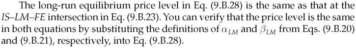
The demand for labor is based on the marginal product of labor, as determined by the production function. Recall from Chapter 3 (Eq. 3.1) that the production func­tion can be written as Y = AF (K, N), where Y is output, K is the capital stock, N is labor input, and A is productivity. Holding the capital stock K fixed, we can write the production function with output Y as a function only of labor input N and productivity A. A useful specific production function is

where f₁ and f₂ are positive numbers.

The marginal product of labor, MPN, is the slope of the production function. The slope of the production function in Eq. (9.B.1) at any level of employment N equals^[CLXII] A( f₁ — f₂ N), so the marginal product of labor is

Firms hire labor to the point at which the marginal product of labor equals the real wage. Thus the relation between the real wage, w, and the amount of labor demanded, ND, is

The supply of labor is an increasing function of the current, after-tax real wage.

where NS is the amount of labor supplied, and n_w is a positive number. Factors other than the after-tax real wage that affect labor supply, such as wealth or the working-age population, are captured by the constant term n 0 in Eq. (9.B.4).

Equilibrium in the Labor Market

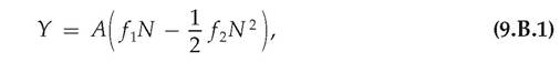
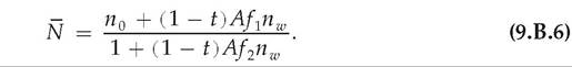
In equilibrium, the amounts of labor demanded, ND, and supplied, NS, are equal; their common value is the full-employment level of employment, N. If we substi­tute N for NS and ND in Eqs. (9.B.3) and (9.B.4), we have two_linear equations in the two variables N and w. Solving these equations for w and N yields²

and

Using the full-employment level of employment,in Eq. (9.B.6), we obtain the full-employment level of output, Y, by substituting N into the production function (9.B.1):

The value of full-employment output in Eq. (9.B.7) is the horizontal intercept of the FE line.

We use these equations to analyze the effects on the labor market of changes in productivity and labor supply. First consider an increase in productivity A. Equation (9.B.5) shows that an increase in A leads to an increase in the equilibrium

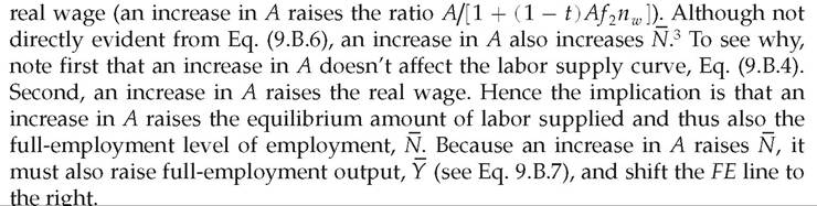
Now consider an increase in the amount of labor supplied at each level of the after-tax real wage, represented algebraically as an increase in n ₀ in Eq.

The Goods Market

To find equilibrium in the goods market, we start with equations describing desired consumption and desired investment. Desired consumption is

where Y — T is disposable income (income Y minus taxes T), r is the real interest rate, and c₀, c_Y, and c_r are positive numbers. The number c_γ in Eq. (9.B.8) is the marginal propensity to consume, as defined in Chapter 4; because people con­sume only part of an increase in disposable income, saving the rest, a reasonable assumption is that 0 < c_γ < 1. According to Eq. (9.B.8), an increase in disposable income causes desired consumption to increase, and an increase in the real interest rate causes desired consumption to fall (and desired saving to rise). Other factors that affect desired consumption, such as wealth or expected future income, are included in the constant term c ₀.⁴

Taxes in Eq. (9.B.8) are

where t is the tax rate on income (the same tax rate that is levied on wages) and t₀ is a lump-sum tax. As mentioned earlier, 0 ≤ t < 1, so an increase in income, Y, increases total taxes, T, and also increases disposable income, Y — T.

Desired investment is

where i₀ and i_r are positive numbers. Equation (9.B.10) indicates that desired investment falls when the real interest rate rises. Other factors affecting desired investment, such as the expected future marginal product of capital, are included in the constant term i ₀.

Equilibrium in the Goods Market

The goods market equilibrium condition in a closed economy is given by Eq. (4.7), which we repeat here:

Equation (9.B.11) is equivalent to the goods market equilibrium condition, S^d = I^d, which could be used equally well here.

If we substitute the equations for desired consumption (Eq. 9.B.8, with taxes T as given by Eq. 9.B.9) and desired investment (Eq. 9.B.10) into the goods market equilibrium condition (Eq. 9.B.11), we get

^[I]Because an increase in taxes, T, reduces desired consumption in Eq. (9.B.8), this formulation of desired consumption appears, at first glance, to be inconsistent with the Ricardian equivalence proposition discussed in Chapter 4. However, essential to the idea of Ricardian equivalence is that consumers expect an increase in current taxes, T, to be accompanied by lower taxes in the future. This decrease in expected future taxes would increase desired consumption, which would be captured in Eq. (9.B.8) as an increase in c ₀. According to the Ricardian equivalence proposition, after an increase in T with no change in current or planned government purchases, an increase in c₀ would exactly offset the reduction in c_Y (Y — T) so that desired consumption would be unchanged.

Collecting the terms that multiply Y on the left side yields

Equation (9.B.13) relates output, Y, to the real interest rate, r, that clears the goods market.

In Eq. (9.B.14), n_is and β_ιs are positive numbers defined as

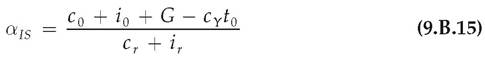
and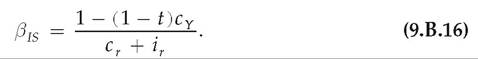

Equation (9.B.14) yields the graph of the IS curve. In Eq. (9.B.14), the coeffi­cient of Y, or — β_ιs, is the slope of the IS curve; because this slope is negative, the IS curve slopes downward. Changes in the constant term n_is in Eq. (9.B.14), which is defined in Eq. (9.B.15), shift the IS curve. Anything that increases α_is—such as (1) an increase in consumer optimism that increases desired consumption by increas­ing c 0; (2) an increase in the expected future marginal product of capital, MPK^f, that raises desired investment by raising i 0; or (3) an increase in government pur­chases, G—shifts the IS curve up and to the right. Similarly, anything that decreases a_IS shifts the IS curve down and to the left.

The Asset Market

In general, the real demand for money depends on real income, Y, and the nominal interest rate on nonmonetary assets, i, which in turn equals the expected real inter­est rate, r, plus the expected rate of inflation, π^e. We assume that the money demand function takes the form

where M^d is the nominal demand for money, P is the price level, and I_γ and I_r are positive numbers. The constant term I0 includes factors other than output and the interest rate that affect money demand, such as the liquidity of alternative assets.

Equilibrium in the Asset Market

As we showed in Chapter 7, if we assume that there are only two types of assets (money and nonmonetary assets), the asset market is in equilibrium when the real quantity of money demanded equals the real money supply, M∣P. Using the money demand function in Eq. (9.B.17), we write the asset market equilibrium condition as

For fixed levels of the nominal money supply, M, price level, P, and expected rate of inflation, π^e, Eq. (9.B.18) relates output, Y, and the real interest rate, r, that clears the asset market. Thus Eq. (9.B.18) defines the LM curve. To get Eq. (9.B.18) into a form that is easier to interpret graphically, we rewrite the equation with r alone on the left side:

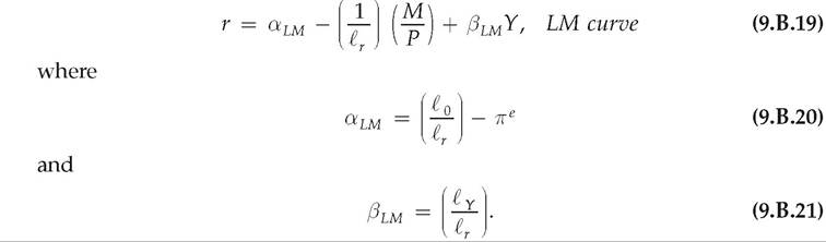
The graph of Eq. (9.B.19) is the LM curve. In Eq. (9.B.19), the coefficient of Y, or e_LM, is the slope of the LM curve; because this coefficient is positive, the LM curve slopes upward. Variables that change the intercept of the equation in Eq. (9.B.19), a_LM — (1 Ó ) (M/P), shift the LM curve. An increase in the real money supply, M/P, reduces this intercept and thus shifts the LM curve down and to the right. An increase in the expected rate of inflation π^e reduces α_lm and shifts the LM curve down and to the right. An increase in real money demand arising from (for example) reduced liquidity of alternative assets raises T₀, which raises α_lm and shifts the LM curve up and to the left.

General Equilibrium in the IS-LM Model From the supply-and-demand relationships and equilibrium conditions in each market, we can calculate the general equilibrium values for the most important macroeconomic variables. We have already solved for the general equilibrium lev­els of the real wage, employment, and output in the labor market: The real wage is given by Eq. (9.B.5); employment equals its full-employment level, N, given by Eq. (9.B.6); and, in general equilibrium, output equals its full-employment level, Y, as given by Eq. (9.B.7).

Turning to the goods market, we obtain the general equilibrium real interest rate by substituting Y for Y in Eq. (9.B.14):

Having output, Y, and the real interest rate, r (determined by Eq. 9.B.22), we use Eqs. (9.B.9), (9.B.8), and (9.B.10) to find the general equilibrium values of taxes, T, consumption, C, and investment, I, respectively.

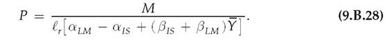
The final important macroeconomic variable whose equilibrium value needs to be determined is the price level, P. To find the equilibrium price level, we work with the asset market equilibrium condition, Eq. (9.B.18). In Eq. (9.B.18), we substi­tute full-employment output, Y, for Y and use Eq. (9.B.22) to substitute the equilib­rium value of the real interest rate for r. Solving Eq. (9.B.18) for the price level gives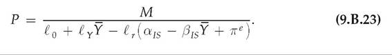

Equation (9.B.23) confirms that the equilibrium price level, P, is proportional to the nominal money supply, M.

We can use these equations to analyze the effects of an adverse productivity shock on the general equilibrium, as in the text. We have already shown that an increase in the productivity parameter, A, increases the equilibrium real wage, the full-employment level of employment, and the full-employment level of output. Thus an adverse productivity shock (a reduction in A) reduces the general equilib­rium levels of the real wage, employment, and output^Equation (9.B.22) indicates that an adverse productivity shock because it reduces Y, must increase the equilib­rium real interest rate. Lower output and a higher real interest rate imply that both consumption and investment must decline (Eqs. 9.B.8 and 9.B.10). Finally, the decrease in Y resulting from an adverse productivity shock reduces the denomi­nator of the right side of Eq. (9.B.23), so the price level, P, must rise. All these results are the same as those found by graphical analysis.

The AD-AS Model

Building on the algebraic version of the IS-LM model just derived, we now derive an algebraic version of the AD-AS model presented in this chapter. We present algebraic versions of the aggregate demand (AD) curve, the short-run aggregate supply (SRAS) curve, and the long-run aggregate supply (LRAS) curve and then solve for short-run and long-run equilibria.

The Aggregate Demand Curve

Aggregate output demanded at any price level, P, is the amount of output corre­sponding to the intersection of the IS and LM curves. We find the value of Y at the intersection of the IS and LM curves by setting the right sides of Eqs. (9.B.14) and (9.B.19) equal and solving for Y:

Equation (9.B.24) is the aggregate demand curve. For constant nominal money supply, M, Eq. (9.B.24) shows that the aggregate quantity of goods demanded, Y, is a decreasing function of the price level, P, so that the AD curve slopes down­ward. Note that the numerator of the right side of Eq. (9.B.24) is the intercept of the IS curve minus the intercept of the LM curve. Thus for a constant price level, any change that shifts the IS curve up and to the right (such as an increase in the government purchases) or shifts the LM curve down and to the right (such as an increase in the nominal money supply) increases aggregate output demanded and shifts the AD curve up and to the right.

The Aggregate Supply Curve

In the short run, firms supply the output demanded at the fixed price level, which we denote P_sr. Thus the short-run aggregate supply (SRAS) curve is a horizontal line:

The long-run aggregate supply curve is a vertical line at the full-employment level of output, Y, or

Short-Run and Long-Run Equilibrium

The short-run equilibrium of the economy is represented by the intersection of the aggregate demand (AD) curve and the short-run aggregate supply (SRAS) curve. We find the quantity of output in short-run equilibrium simply by substituting the equation of the SRAS curve (Eq. 9.B.25) into the equation of the AD curve (Eq. 9.B.24) to obtain

The long-run equilibrium of the economy, which is reached when the labor, goods, and asset markets are all in equilibrium, is represented by the intersection of the aggregate demand curve and the long-run aggregate supply curve. Thus Y = Y in long-run equilibrium, from the LRAS curve in Eq. (9.B.26). We find the price level in long-run equilibrium by setting the right sides of the equation of the AD curve (Eq. 9.B.24) and the equation of the LRAS curve (Eq. 9.B.26) equal and solv­ing for P to obtain