Appendix F: Random Variables and Stochastic Processes

This appendix introduces the concepts of probability, random variables, and stochastic processes. Such concepts are extremely useful for analyzing macroeconomic models characterized by uncertainty.

F.1 Probability

Probability is the measure of the likelihood that an event will occur. Probabilities are quantified as real numbers between 0 and 1, where, loosely speaking, 0 indicates impossibility and 1 indicates certainty. The higher the probability of an event, the more likely it is that the event will occur.

A simple example is the tossing of a fair (unbiased) coin. Because the coin is fair, the two outcomes (“heads” and “tails”) are both equally probable. The probability of heads equals the probability of tails. Because no other outcomes are possible, the probability of either heads or tails is 1/2, which can also be written as 0.5 or 50%.

The concepts discussed here have been given an axiomatic mathematical formalization in probability theory, which is used widely in many areas of applied study, including economics.

The mathematical theory of probability has its roots in attempts to analyze games of chance by Gerolamo Cardano in the sixteenth century and by Pierre de Fermat and Blaise Pascal in the seventeenth century. Christiaan Huygens published a book on the subject in 1657, and in the nineteenth century, Pierre Laplace completed what is today considered the classic interpretation of probability.

Initially, probability theory mainly considered discrete events, and its methods were mainly combinatorial. Eventually, analytical considerations compelled the incorporation of continuous variables into the theory. This effort culminated in modern probability theory, based on foundations laid by Andrey Nikolaevich Kolmogorov.

Although probability is interpreted in several different ways, probability theory treats the concept in a rigorous mathematical manner by expressing it through a set of axioms. Typically these axioms formalize probability in terms of a probability space, which assigns a measure taking values between 0 and 1, termed the probability measure, to a set of outcomes called the sample space. Any specified subset of these outcomes is called an event.

Central subjects in probability theory include discrete and continuous random variables, probability distributions, and stochastic processes. These concepts provide mathematical abstractions of nondeterministic or uncertain processes or measured quantities that may either be single occurrences or evolve over time in a random fashion.

F.2 Random Variables and Probability Distributions

A random variable (or stochastic variable) is a variable whose possible values are outcomes of a random phenomenon. A random variable is defined as a function that maps outcomes to numerical quantities, typically real numbers. A random variable has a probability distribution, which specifies the probability that its value falls in any given interval.

Random variables can be discrete or continuous. Discrete random variables take any of a specified finite or countable list of values, and they are endowed with a probability mass function characteristic of the random variable’s probability distribution. Continuous random variables take any numerical value in an interval or collection of intervals, via a probability density function, which is characteristic of the random variable’s probability distribution. Random variables can also be a mixture of both types.

The formal mathematical treatment of random variables is a topic in probability theory.

F.2.1 Discrete Probability Distributions

Discrete probability theory deals with events that occur in countable sample spaces, such as tossing a coin, throwing dice, or experiments with decks of cards.

Initially, the probability of an event was defined as the number of cases in which the event occurred, divided by the number of total outcomes possible in an equiprobable sample space.

The modern axiomatic definition starts with a finite or countable set called the sample space, which relates to the set of all possible outcomes, denoted by Ω. It is then assumed that for each element x ∈ Ω, one can attach an intrinsic probability value f(x), which satisfies the following properties:

The probability function f(x) lies between zero and one for every value of x in the sample space Ω, and the sum of f(x) over all values of x in the sample space Ω is equal to 1.

An event is defined as any subset E of the sample space Ω. The probability of the event E is defined as

Therefore, the probability of the entire sample space is 1, and the probability of the null event is 0. The function f(x), mapping a point in the sample space to the probability value, is called a probability mass function.

F.2.2 Continuous Probability Distributions

Continuous probability theory deals with events that occur in a continuous sample space. If the outcome space of a random variable X is the set of real numbers ℝ or a subset thereof, then a function F can be defined so as to satisfy

Such a function is called a cumulative distribution function (CDF) and returns the probability that X will be less than or equal to x.

The CDF F is a monotonically nondecreasing right continuous function that satisfies the following two properties:

If F is continuous everywhere (i.e., its derivative exists and integrating the derivative gives us the CDF back again), then the random variable X is said to have a probability density function PDF, or simply density f(x), which is defined as the first derivative of the cumulative distribution function F(x):

For a set E that is a subset of ℝ, the probability of a random variable being in E is given by

If the PDF exists, then the above can be written as

Whereas the PDF exists only for continuous random variables, the CDF exists for all random variables (including discrete random variables) that take values in ℝ. These concepts can be generalized for multidimensional cases on ℝⁿ and other continuous sample spaces.

F.2.3 Mathematical Expectation, Variance, and Higher Moments

In probability theory, the expected value of a random variable is, intuitively, the long-run average value of repetitions of the experiment it represents. For example, the expected value in rolling a six-sided die is 3.5, because the average of all the numbers that come up in an extremely large number of rolls is close to 3.5. The expected value is also known as the mathematical expectation, mean value, mean, or first moment of the random variable.

The expected value of a discrete random variable is the probability-weighted average of all possible values. In other words, each possible value that the random variable can assume is multiplied by its probability of occurring, and the resulting products are summed to produce the expected value.

The mathematical expectation of a discrete random variable is defined as

For a continuous random variable, it is defined as

The expected value is a key aspect of how one characterizes a probability distribution. It is one type of location parameter.

By contrast, the variance is a measure of dispersion of the possible values of the random variable around the expected value. The variance itself is defined in terms of two expectations: It is the expected value of the squared deviation of the variable’s value from its expected value. For a discrete random variable, it is defined as

For a continuous random variable, it is defined as

Third and higher moments can be defined accordingly and are measures of the skewness and kurtosis of probability distributions. The first and second moments, as used in the mean and variance, are examples of low-order statistics.

F.2.4 Some Useful Probability Distributions

Certain probability distributions occur very often in probability theory, because they are deemed to be good descriptions of many natural or physical processes. Their distributions therefore have gained special importance in probability theory.

Some fundamental discrete distributions are the discrete uniform, Bernoulli, binomial, negative binomial, Poisson, and geometric distributions.

Let us briefly discuss a few of these probability distributions.

The discrete uniform distribution is a symmetric probability distribution whereby a finite number of values are equally likely to be observed. Every one of n values has equal probability 1/n. Another way of describing it would be that a known, finite number of outcomes are equally likely to happen.

A simple example of the discrete uniform distribution is throwing a fair die. The possible values are 1, 2, 3, 4, 5, 6, and each time the die is thrown, the probability of a given score is 1/6.

The discrete uniform distribution itself is inherently nonparametric. It is convenient, however, to represent its values generally by all integers in an interval [a, b], so that a and b become the main parameters of the distribution. Often one simply considers the interval [1, n] with the single parameter n. With these conventions, the CDF of the discrete uniform distribution can be expressed, for any x ∈ [a, b], as

The expected value of a uniformly distributed discrete random variable X, with n integers in the interval [a, b], is given by

The variance is given by

The Bernoulli distribution, named after the Swiss scientist Jacob Bernoulli, is the probability distribution of a random variable that takes the value 1 with probability p and the value 0 with probability q = 1 − p.

The expected value of a Bernoulli random variable X is given by

The variance of a Bernoulli random variable X is given by

We next move to continuous distributions. The continuous uniform distribution or rectangular distribution is a family of symmetric probability distributions such that for each member of the family, all intervals of the same length on the distribution’s support are equally probable. It is the continuous equivalent of the discrete uniform distribution. The support is defined by two parameters, a and b, which are the distribution’s minimum and maximum values. The distribution is often referred to by the expression U(a, b).

The probability density function of the continuous uniform distribution is given by

The probability density function of the continuous uniform distribution is presented in figure F.1 for three values of the support [a, b].

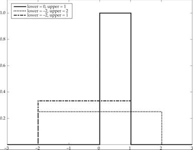
Figure F.1 The uniform distribution.

For a = 0 and b = 1, the resulting distribution U(0, 1) is called the standard uniform distribution. The standard uniform distribution is also depicted in figure F.1.

The mean and variance of the uniform distribution are given by

The probability that a uniformly distributed random variable falls within any interval of fixed length is independent of the location of the interval itself; it is only dependent on the interval size, so long as the interval is contained in the distribution’s support.

To see this, if X ∼ U(a, b), and [x, x + d] is a subinterval of [a, b] with fixed d > 0, then

which is independent of x. In fact, this is what motivates the distribution’s name.

The CDF of the continuous uniform distribution is given by

The CDF of the continuous uniform distribution is depicted in figure F.2.

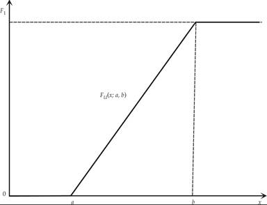
Figure F.2 The CDF of the continuous uniform distribution.

As a final example, let us consider the normal distribution. The probability density function of this distribution is given by

where μ is the mean of the distribution, and σ² is its variance.

The special case when μ = 0 and σ² = 1 is known as the standard normal distribution. It is given by

This special case is depicted in figure F.3, along with two other normal distributions with higher variances.

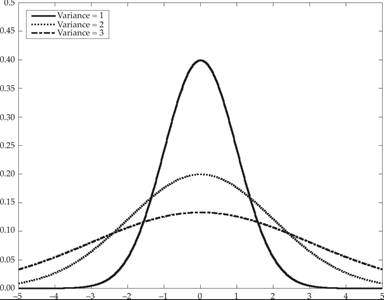
Figure F.3 The normal distribution.

The factor in the denominator ensures that the total area under the curve is equal to one. The factor 1/2 in the exponent ensures that the distribution has unit variance and therefore also has unit standard deviation. This function is symmetric around x = 0, where it attains its maximum value, and it has inflection points at x = 1 and x = −1.

In fact, every normal distribution is a version of the standard normal distribution whose domain has been stretched by a factor σ and moved in a parallel fashion by μ. The relationship between the general normal distribution and the standard normal distribution is given by

The PDF must be scaled by 1/σ so that the integral is still 1.

The CDF of the standard normal distribution, often denoted by Φ, is given by

The CDF of the standard normal distribution is depicted in figure F.4.

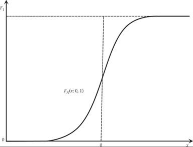
Figure F.4 The CDF of the standard normal distribution.

The normal distribution is extremely important because of the central limit theorem. In its most general form, this theorem states that under some conditions (which include a finite variance), averages of samples of observations of random variables that are independently drawn from independent distributions, converge in distribution to the normal. In other words, the averages become normally distributed when the number of observations is sufficiently large.

The central limit theorem is one of two major results in probability theory providing some structure for random events. The second is the law of large numbers, which is discussed in subsection F.2.6.

To understand these results, we must first discuss the different concepts of convergence of random variables.

F.2.5 Convergence of Random Variables

In probability theory, there are several notions of convergence for random variables. They are listed below in order of strength, ranging from weak to strong convergence.

Weak convergence: A sequence of random variables X₁, X₂, …, converges weakly to a random variable X if their respective cumulative distribution functions F₁, F₂, …, converge to the cumulative distribution function F of X, wherever F is continuous. Weak convergence is also called convergence in distribution.

Convergence in probability: A sequence of random variables X₁, X₂, …, converges in probability to the random variable X if

for every ε > 0.

Strong convergence: A sequence of random variables X₁, X₂, …, converges strongly to the random variable X if

Strong convergence is also known as almost sure convergence.

F.2.6 The Law of Large Numbers

Intuition suggests that if a fair coin is tossed many times, then roughly half of the time, it will turn up heads, and the other half, it will turn up tails. Furthermore, the more often the coin is tossed, the more likely it should be that the ratio of the number of heads to the number of tails will approach unity.

Modern probability theory provides a formal version of this intuitive idea, known as the law of large numbers. This law is remarkable, because it is not assumed in the foundations of probability theory but instead emerges from these foundations as a theorem. Because it links theoretically derived probabilities to their actual frequency of occurrence in the real world, the law of large numbers is considered a pillar in the history of statistical theory and has been widely influential.

The law of large numbers states that the sample average of a sequence of independent and identically distributed random variables X_k converges toward their common expectation μ, provided that the expectation of |X_k| is finite.

The sample average is defined as

The weak law of large numbers is based on convergence in probability. It states that

The strong law of large numbers is based on almost sure convergence. It states that

F.2.7 The Central Limit Theorem

The central limit theorem is one of the great results of mathematical statistics. It explains the ubiquitous occurrence of the normal distribution in nature. The theorem states that the average of many independent and identically distributed random variables with finite variance tends toward a normal distribution, irrespective of the distribution followed by the original random variables.

Formally, let X₁, X₂, …, be independent random variables with mean μ and variance σ² > 0. Then the sequence of random variables

converges in distribution to the standard normal variable.

For some classes of random variables—for example, the distributions with finite first, second, and third moments from the exponential family—the classic central limit theorem works rather fast. However, for some random variables of the heavy tail and fat tail variety, it works very slowly or may not work at all: in such cases, one may use the generalized central limit theorem.

F.2.8 Joint Probability Distributions

Up to now we have dealt with probability distributions of a single random variable. Given at least two random variables X, Y, …, that are defined on a probability space, the joint probability distribution for X, Y, … is a probability distribution that gives the probability that each of X, Y, … falls in any particular range or discrete set of values specified for that variable. In the case of only two random variables, this is called a bivariate distribution, but the concept generalizes to any number of random variables, giving a multivariate distribution.

The joint probability distribution can be expressed either in terms of a joint cumulative distribution function or in terms of a joint probability density function (in the case of continuous variables) or joint probability mass function (in the case of discrete variables). These in turn can be used to find two other types of distributions: the marginal distribution, giving the probabilities for any one of the variables with no reference to any specific ranges of values for the other variables; and the conditional probability distribution, giving the probabilities for any subset of the variables conditional on particular values of the remaining variables.

The joint probability mass function of two discrete random variables X, Y is given by

where P(X = x|Y = y) is the conditional probability mass function, which gives the probability that X = x, conditional on the fact that Y = y; P(Y = y) is the marginal probability mass function, giving the probability that Y = y, irrespective of X. The other conditional and marginal probabilities are defined similarly.

The property that a joint probability distribution can be expressed as the product of the relevant conditional and marginal distributions generalizes to any number of variables n and is known as the chain rule of probability. Joint probability density functions for continuous variables are defined accordingly.

A useful measure of the joint variability of two random variables is the covariance. The covariance between two jointly distributed real-valued random variables X and Y, with finite second moments, is defined as the expected product of their deviations from their individual expected values:

If higher values of one variable mainly correspond with higher value of the other variable, and the same holds for lower values (i.e., if the variables tend to show similar behavior), then the covariance is positive. In the opposite case, when the higher values of one variable mainly correspond to lower values of the other (i.e., the variables tend to show opposite behavior), then the covariance is negative. The sign of the covariance therefore shows the tendency in the linear relationship between the variables.

The magnitude of the covariance is not easy to interpret. The normalized version of the covariance, the correlation coefficient, however, shows by its magnitude the strength of the linear relation. The correlation coefficient, due to Pearson, is the covariance of two random variables divided by the product of their standard deviations and is unit free. The correlation coefficient ranges from −1 to 1.

F.3 Stochastic Processes

A stochastic process or random process can be defined as a collection of random variables that is indexed by some mathematical set, meaning that each random variable of the stochastic process is uniquely associated with an element in the set. The set used to index the random variables is called the index set. Historically, the index set was some subset of the real line, such as the natural numbers, giving the index set the interpretation of time. Each random variable in the collection takes values from the same mathematical space known as the state space. This state space can be, for example, the integers, the real line, or n-dimensional Euclidean space.

An increment is the amount that a stochastic process changes between two index values (often interpreted as two points in time). A stochastic process can have many outcomes, due to its randomness, and a single outcome of a stochastic process is called, among other names, a sample function or realization.

Thus, for our purposes, a stochastic process will be defined as a collection of random variables evolving over time. It is a process that evolves over time according to probabilistic rules.

Dynamic stochastic models can be contrasted with deterministic models. A deterministic model is specified by a set of differential or difference equations that describe exactly how the system will evolve over time. In a stochastic model, the evolution is at least partially random, and if the process is run several times, it will not give identical results. Different runs of a stochastic process are different realizations of the process.

Thus, instead of describing a process that can evolve in only one way, as in the case of solutions of systems of ordinary differential or difference equations, in a stochastic process, there is potential indeterminacy. Even if the initial conditions (or starting points) are known, there are several (often infinitely many) directions in which the process can evolve.

Like random variables, stochastic processes can be defined in both continuous and discrete time. In the case of discrete time, a stochastic process is a sequence of random variables. The random variables corresponding to various time periods may be completely different, the only requirement being that these different random quantities all take values in the same space. The approach we take is to model these random variables as random functions of the time index. Although the random values of a stochastic process at different times may be independent random variables, in most commonly considered situations, they exhibit complicated statistical dependence.

In the remainder of this appendix, let us confine our attention to linear stochastic processes in discrete time. Such processes are extremely useful tools for studying dynamic stochastic economic problems that combine time and randomness. Aggregate fluctuations are an important example of the application of these tools.

As Lucas [1977, p. 9] observed: “Movements about trend in gross national product in any country can be well described by a stochastically disturbed difference equation of very low order.” Stochastically disturbed difference equations are nothing more than difference equations that are affected by random shocks. They are examples of stochastic processes in discrete time.

F.4 Univariate Linear Stochastic Processes in Discrete Time

A stochastic process y_t is defined as a collection of random variables that depend on the time index. One random variable corresponds to each moment of time t ∈ T.

Assume that the probability law that corresponds to each stochastic process is characterized by the set of mathematical expectations (means) of the stochastic process y_t and by the set of covariances of y in different time periods.

The mathematical expectation (or mean) of the stochastic process y_t is given by

for t ∈ T, where E is the mathematical expectations operator.

The covariances are given by

A stochastic process is considered stationary when the mean μ_t is independent of t, and the covariance σ_{t, s} only depends on t − s.

F.4.1 The White Noise Process

The basic stochastic process, which is the building block of all the stochastic processes that we analyze here, is the white noise process. In this process, the mean is equal to zero, the variance is constant, and the covariance is equal to zero for t≠s.

Thus, the white noise process ε satisfies the following properties:

In the white noise process, there is no time dependence, as the covariances are equal to zero for different time periods. Zero mean normal distributions are examples of white noise processes, as are uniform distributions with support [−a, a].

F.4.2 Moving Average Stochastic Processes

Another category of linear stochastic processes in discrete time is the category of moving average processes. The first-order moving average stochastic process (MA(1)) is defined by

where ε_t is a white noise process.

For this process, it follows that

It is straightforward to confirm that this stochastic process is stationary.

A more general linear moving average stochastic process can be defined as

where Θ(L) is an nth-order polynomial in the lag operator L. Equation (F.2) defines an MA(n) stochastic process.

F.4.3 Autoregressive Stochastic Processes

Another category of linear stochastic processes is the category of autoregressive stochastic processes.

The zero mean first-order linear autoregressive process AR(1) is defined by

where λ ≤ 1, and ε_t is a white noise process.

An AR(1) process (F.3) is essentially a stochastic first-order difference equation (i.e., a first-order difference equation plus a white noise stochastic process).

Using the lag operator, it follows that

We can deduce that this stochastic process has the white noise process ε as its building block. Equation (F.3) is the moving average representation of the AR(1) process (F.4). Thus the AR(1) process is an example of an infinite-order moving average process with geometrically declining weights. It follows that

The AR(1) process is stationary if |λ| < 1. If |λ|≥ 1, this AR(1) process is nonstationary.

In the case λ = 1, it is nonstationary and takes the form

The nonstationary stochastic process (F.5) is called a random walk. The first difference of a random walk is a white noise process, because from (F.5), it follows that

where Δ is the first difference operator.

The random walk is a special case of the class of homogeneous nonstationary stochastic processes, which become stationary when we transform them by taking their first differences one or more times.

The second-order linear autoregressive process (AR(2)) has the form of a second-order linear difference equation plus a white noise stochastic process:

where ε_t is a white noise process, and a, b, c are constant parameters. Using the lag operator, (F.7) can be rewritten as

Equation (F.8) can be transformed into

where λ₁ + λ₂ = b and λ₁λ₂ = −c are the two roots of the characteristic polynomial of the difference equation (F.7).

The conditions for (F.7) to be stationary are analogous to the conditions for convergence in a standard second-order linear difference equation. There are three possible cases.

Case 1 b² > −4c The roots are real and distinct, and they take the form

We have stationarity if |λ₁| < 1, and |λ₂| < 1. The solution takes the form

Case 2 b² = −4c We have two equal real roots of the form

We have stationarity if |λ| < 1, which requires |b| < 2.

Case 3 b² < −4c We have two complex roots, which take the form of a pair of complex conjugates. We have stationarity if |c| < 1, which also implies in this case that |b| < 2.

A more general autoregressive process AR(m) takes the form

where Λ(L) is a polynomial in the lag operator.

F.4.4 Autoregressive Moving Average Stochastic Processes

Autoregressive and moving average processes can be combined. For example, the combined first-order autoregressive moving average process is called ARMA(1,1) and is defined by

This ARMA process is stationary if |λ| < 1.

For a more general and detailed treatment of linear stochastic processes in discrete time, see chapter 11 in Sargent [1987].

F.5 Vector Stochastic Processes and Vector Autoregressions

Let us now consider the following system of n first-order stochastic difference equations. Such systems arise quite often in dynamic macroeconomics and are a generalization of the deterministic system of difference equations examined in appendix D:

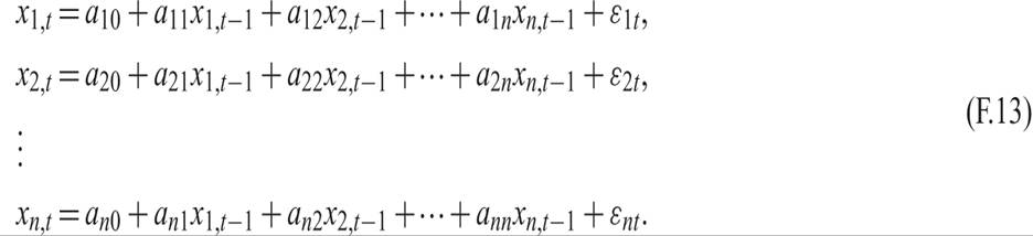
The xs are observable variables, and the εs are white noise stochastic disturbances. Such a system is called a vector autoregression and is a widely used example of a vector stochastic process.

In matrix form, the system (F.13) can be written as

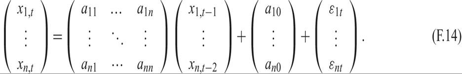
By defining the vector of xs as x, the matrix of multiplicative parameters as A, the vector of the constants as a₀, and the vector of the disturbances as e, the system can be written as

The coefficient matrix A can be transformed as

where J is a diagonal matrix with the eigenvalues of A on the diagonal, and P is a matrix consisting of the corresponding (right) eigenvectors.

This vector stochastic process is stationary if all eigenvalues of A are inside the unit circle. Sims [1980] pioneered the use of vector autoregressions as a theory-free way of modeling dynamic interactions between macroeconomic time series. Since then, vector autoregressions have become a widely used tool in empirical macroeconomics.

1. This is a review meant for readers who have already taken courses in mathematical statistics. As a result, it is neither comprehensive nor fully rigorous. For a fuller treatment, consult a comprehensive text on mathematical statistics, such as Larsen and Marx [2014].