Appendix E: Methods of Intertemporal Optimization

Optimization in dynamic economic problems, which are problems in which variables change over time, does not require new principles vis-à-vis static problems. However, dynamic problems have a special structure that allows us to say more about their solution methods.

The most important part of this special structure is the relation between stocks and flows. Some variables, which we shall denote by y, have the form of stocks, changing gradually over time. Other variables, which we shall denote by x, have the form of flows, which can change freely at any instant. In mathematical terminology, stocks are called state variables, and flows are called control variables.

In this appendix, we briefly review methods of intertemporal optimization.¹

E.1 The Form of Dynamic Optimization Problems

The change in stocks depends on the evolution of both stocks and flows. Mathematically, control variables control changes in state variables. For example, savings in period t determine the change in household wealth from period t to period t + 1. The determination of the evolution of state variables has the form

where t, t + 1, … are discrete time periods, y is a state variable (stocks), x is a control variable (flows), and Q is a vector function.

Apart from the restrictions that determine the evolution of state variables, there may be other restrictions between all variables that refer to a specific time period. Such restrictions take the form

where G is a vector function.

In most dynamic economic problems, we assume that economic agents optimize an objec-tive function of the form

subject to restrictions of the form of (E.1) and (E.2).

Note that the period of optimization begins at t = 0 and ends at t = T. The value of the initial stock in period 0 is taken as given, and the same applies to the value of stocks in period T + 1. One needs an initial and a final, or transversality, condition to solve such problems.

E.2 The Method of Optimal Control

The problem is to select the variables y_t and x_t for t = 0, 1, 2, …, T, to find the optimal solution of (E.3) under the constraints (E.1) and (E.2).

One can define multipliers (shadow values) and construct the Lagrange function. Define as μ_t the multipliers for the constraints (E.2). These have the usual interpretation of shadow values for the constraints in period t. The multipliers (shadow values) for the constraints (E.1) are different from those of the static constraints. They define the first-order change in the objective function if the constraint in the change of the stock is loosened (i.e., if we have a marginal increase in the stock variable y_t+1). Thus, they are the shadow values of the stock variables in period t + 1, and we denote them by λ_t+1.

We define as ℒ the Lagrange function of the full intertemporal problem:

The first-order conditions for the optimization of the Lagrange function with respect to the control variables x are relatively straightforward:

for t = 0, 1, …, T, where F_x, Q_x, G_x denote the first derivative of the relevant functions with respect to x.

With respect to the state variables y, the first-order conditions are more complex, because each y appears in two terms of the sum: in the term for period t and also in the term for period t− 1.

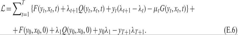
The final four terms in (E.6) refer to y₀ and y_T+1 which are taken as given. The first-order conditions for the optimum of ℒ, for y_t, t = 1, 2, …, T are

Equation (E.7) can be written as

These conditions can be written in a more comprehensive and economically useful way. Define a new function, the Hamilton function ℋ, as follows:

Equation (E.5) suggests that the control variables x must be selected to optimize ℋ(y, x, λ, t), under the constraint G(y, x, t) ≤ 0.

Define the rearranged Lagrange function in the following way:

Then (E.8) can be written more simply as

Finally, from (E.1) and (E.9), taking into account the envelope theorem, we get

These properties of the Hamilton function are summarized in the maximum principle.

Maximum Principle The necessary first-order conditions for the optimization of (E.3), under the constraints (E.1) and (E.2), are the following: (1) For each t, the control variables x_t optimize the Hamilton function (E.9) under the static constraints (E.2).

The maximum principle, which was proposed by Pontryagin et al. [1962], greatly facilitates the determination of the first-order conditions for intertemporal optimization problems. In addition, it also has a great advantage for economic applications, as it facilitates the economic interpretation of the first-order conditions.

Obviously, we do not want the control variables x to optimize the function F, because this would not take into account the impact of the choice of x on the evolution of the state variables y in the next period. The impact is accounted for optimizing (E.9). The impact of x_t on y_t+1 is equal to its impact on Q. The change in the objective function is found by multiplying the impact of x on Q with the shadow value λ_t+1 of y_t+1. The Hamilton function (E.9) accomplishes this. The Hamilton function provides a simple way of converting the one-period objective function F to account for the future impact of the current choice of the control variables x.

A similar economic interpretation can be given to the first-order conditions for the state variable y. A marginal change in y in period t gives the marginal change F_y − μG_y in period t, given the shadow value of the static restriction G, and an additional Q_y in the next period, with a value of λ_t+1. The right-hand side of (E.8) may be interpreted as a dividend. The change λ_t+1 − λ_t is like a capital gain. Equation (E.8) tells us that the dividend plus the capital gain should be equal to zero: At the optimum point, there can be no excess return from y.

E.3 The Optimal Control Method in Continuous Time

Until now we have treated time as a sequence of discrete periods. However, in many applications, it is more convenient to treat time as a continuous variable.

We can think of continuous time as the limit of discrete periods of length Δt, where Δt tends to zero. For example, (E.1) can be written as

Dividing by Δt and letting it tend to zero, we get

where as usual, a dot above a variable denotes its first derivative with respect to time. Let us also use the widespread convention that t is written as a subscript in the analysis of discrete time, and in parentheses in the analysis of continuous time.

Equation (E.2), which denotes the constraints in the control variables, does not change. In continuous time, it is written as

The transformation of the sum (E.3) in continuous time is somewhat more complicated. Total time between 0 and T is divided into T/Δt small discrete time intervals. Equation (E.3) can then be written as

The limit of the above sum, as Δt tends to zero, is the integral

We can use the Hamilton function as we did in (E.9):

The first-order conditions for the optimization of the Hamilton function (E.16) under the static constraints (E.14) are

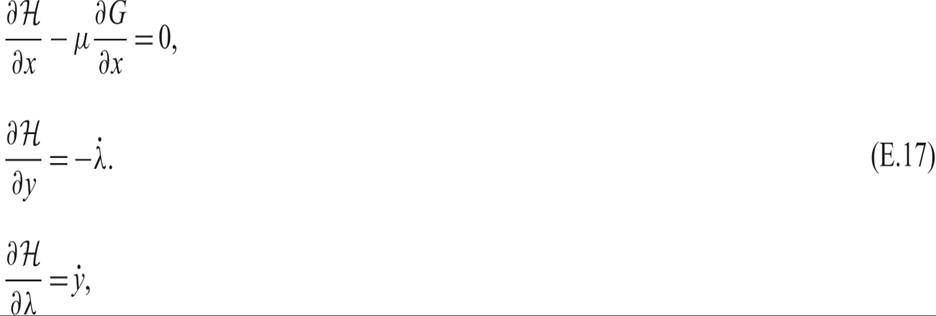
Equations (E.17) are the corresponding conditions in continuous time of the discrete time conditions (E.5), (E.11), and (E.12).

E.4 Dynamic Programming and the Bellman Equation

Dynamic programming is an alternative method of solving the problem of the optimization of a function such as (E.3) under the constraints (E.1) and (E.2).

Our problem is the optimization of

under the constraints

and

for t = 0, 1, 2, …, T. The vectors of initial and final stocks y₀ and y_T+1 are taken as given.

We can define the optimal value that comes out of this problem as a function of the initial stocks y₀. Denote this function as V(y₀). The vector of the first derivatives of this function, V_y(y₀), is the vector of the shadow values of these initial stocks.

The separability of the objective function (E.3) and the constraints allow us to make an important generalization of the above idea. Instead of starting off at time zero, let us assume that we start off at time t = τ. For the decisions that start at τ, the only thing that matters from the past is the vector of stocks y_τ, which is the result of past decisions. Our problem is to optimize an objective function such as (E.3), under the constraints (E.1) and (E.2), with time starting from τ and not from 0. We define V(y_τ, τ) as the optimal value that emerges as a function of stocks y_τ and period τ. The vector of the first derivatives V_y(y_τ, τ) denotes the marginal increase in the optimal value for a small increase of stocks in period τ, which is the vector of shadow values of the initial stocks for the optimization problem that starts in period τ. This applies for all t.

Let us then select any t and examine the decision of choosing the values of the control variables for that period. Any choice of the control variables x_t will lead to stocks y_t+1 through (E.1). What remains is to solve the subproblem for period t + 1, and to find the optimal value V(y_t+1, t + 1). The total value in period t of a choice for the control variables x_t, starting off with stocks y_t, can be separated into two terms: F(y_t, x_t, t), which occurs in the current period; and V(y_t+1, t + 1), which comes about in future periods. The choice of x_t must optimize the sum of these two terms under the relevant constraints. In other words we have

under the constraints (E.1) and (E.2) for the specific t.

This method of intertemporal optimization, as a succession of static optimization problems, was proposed by Richard Bellman and is called dynamic programming. The idea that whatever the choice in period t, the choices for the subproblem that begins from period t + 1 should be optimal, is known as Bellman’s principle of optimality. The optimal value function V(y_t, t) is called the Bellman value function, and equation (E.18) the Bellman equation.

The Bellman equation gives us a recursive method for solving the original optimization problem. The idea is to start from the end and go backward recursively. In period T there is no future, only the requirement for a given final stock y_T+1. Therefore

under the constraints

This is a simple problem of static optimization, which gives us the optimal value function V(y_T, T). This function can in turn be used in the right-hand side of (E.18) for t = T − 1. This equation is then another static problem, which gives us the optimal value function V(y_T−1, T − 1). We can continue in this way, until we reach period 0. In practice, this process provides results for the simplest problems. Analytical solutions exist when the functions F, G, and Q have a very simple form. Where analytical solutions do not exist, we can use numerical solutions.

For many economic applications we have better methods than the recursive method to find or characterize the solution.

Note that in the presence of uncertainty, the Bellman equation (E.18) takes the form

where E is the mathematical expectations operator.

To find the Bellman equation in continuous time, note that from (E.18), we have

where Δt is a small time interval. Using a Taylor expansion of the last right-hand side term of (E.19), we get

From (E.1), we have

Substituting (E.21) in (E.20), and the equation that results in (E.19) yields

Dividing by Δt and noting that V(y(t), t) cancels out from both sides results in

under the static constraint

Equation (E.22) is the Bellman equation for problems in continuous time.

E.5 An Example Based on Optimal Savings in Continuous Time

Let us apply these techniques to one specific example. The example is the Ramsey [1928] problem of the choice of optimal savings in continuous time. This example will also allow us to investigate the role of discounting of the future, which applies to most dynamic optimization problems in economics.

Assume a household that has a exogenous flow of income equal to w per instant and that can borrow and lend freely in the capital market, at an interest rate r. The household has an finite horizon T and initial interest-yielding assets equal to a(0). The household is assumed to maximize the following inter-temporal utility function:

subject to

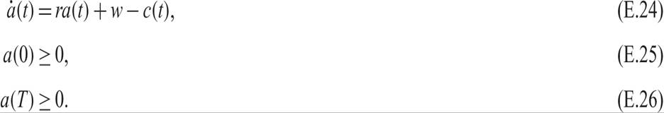
In these equations, u is the instantaneous utility function of the household, which depends on consumption of goods and services and is assumed to be twice differentiable and concave; and ρ is the pure rate of time preference, the rate at which the household discounts future utilities. Equation (E.24) is the instantaneous asset accumulation equation, describing how savings in each instant lead to a change in the assets of the household. Equaion (E.25) defines its initial assets, and (E.26) is a terminal condition that ensures that the household respects its intertemporal budget constraint (transversality condition). Equation (E.26) essentially rules out the possibility that the household has negative assets (i.e., debts) at the end of the horizon.

The Hamilton function for this problem is

where μ is the multiplier of the Hamilton function; μ can be interpreted as the discounted value of marginal assets. Note that because utility at t is discounted, (E.27) is the present-value Hamilton function, viewed from the initial time 0. Correspondingly, μ is the discounted, or present-value multiplier at time 0.

The first-order conditions for a maximum are

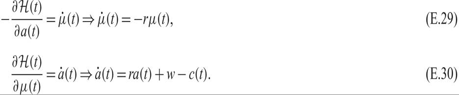
Equation (E.28) implies that at the optimum, the discounted marginal utility of consumption is equal to the discounted marginal value of assets μ. Equation (E.29) implies that the rate of change of the discounted marginal value of assets μ is equal to minus the real interest rate. Equation (E.30) is just the asset accumulation equation.

Conditions (E.25) and (E.26) must be satisfied as well. In fact, (E.26) must be satisfied as an equality. If assets at the end of the horizon were positive, this would not be a maximum, as the household could increase its utility by consuming the remaining assets just before the end of the horizon.

The economic interpretation of these conditions is more intuitive if everything is exp-ressed in current rather than discounted values. Equation (E.28) implies that

where λ(t) is defined as the current value multiplier (i.e., the nondiscounted marginal value of assets at instant t). From (E.31), at the optimum, the current value multiplier λ(t) is the marginal utility of current consumption. From (E.31), it follows that

Substituting the first-order condition (E.29) in (E.32) yields the following first-order condition for the current value multiplier:

From (E.33), along the optimal path, the current marginal value of assets declines at a rate equal to the difference between the real interest rate and the pure rate of time preference of the household. By rearranging (E.33), we get

The real interest rate plus the expected rate of change of the marginal value of assets is equal to the pure rate of time preference. Hence, at the optimum, the household is indifferent between asset accumualation and consumption.

Equations (E.31) and (E.33) express the first-order conditions in terms of the current rather than the discounted value multiplier. These conditions can be derived directly if one forms the current-value Hamilton function:

The conditions for the maximization of the current-value Hamilton function will be the same as the conditions for the maximization of the present-value Hamilton function, as one is a monotonic transformation of the other. These conditions are

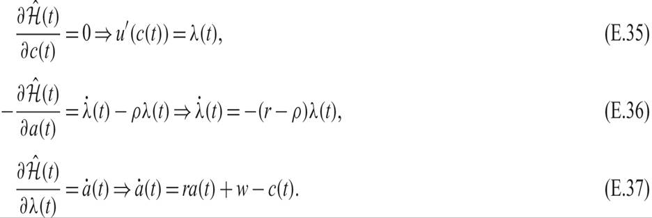
From (E.35), on the optimal path, the multiplier λ(t) (which is the current value of the marginal increase in assets) is equal to the marginal utility of consumption. Thus, the household is indifferent between one extra unit of consumption and one extra unit of savings. From (E.36), on the optimal path, the real interest rate plus the expected capital gain on assets is equal to the pure rate of time preference. Finally, (E.37) is the asset accumulation equation.

Dynamic economic optimization problems usually include discounting. In such problems, one can use the current-value Hamilton function (E.34) and the first-order conditions (E.35)–(E.37), as these first-order conditions are more easily interpretable than the first-order conditions (E.28)–(E.30) for the discounted-value Hamilton function (E.27).

Let us use the first-order conditions (E.35) and (E.36) to characterize the behavior of consumption along the optimal path. From (E.35), differentiating with respect to time, we get

Substituting (E.35) and (E.38) in (E.36) yields

Equation (E.39) is termed the Euler equation for consumption. Because the second derivative of the instantaneous utility function is negative (due to the concavity assumption), the change in consumption will have the same sign as the difference between the real interest rate and the pure rate of time preference. If the real interest rate is higher than the pure rate of time preference, consumption will be continuously increasing. In the opposite case, consumption will be continuously decreasing. If the real interest rate is equal to the pure rate of time preference, consumption will be constant on the optimal path. A full analysis of this dynamic problem is contained in chapter 4. A solution of this problem under uncertainty, using dynamic programming, is contained in chapter 10.

1. This brief review is meant to refresh one’s knowledge and does not aim to be either comprehensive or fully rigorous. Methods of dynamic optimization are fully analyzed in comprehensive texts of mathematics for economists, such as Chiang [1974], Simon and Blume [1994], or Klein [2013]. Some mathematical texts that specialize in intertemporal optimization for economists are also useful such as Intriligator [1971], Kamien and Schwartz [1981], and Dixit [1990].