Appendix D: Difference Equations

In this appendix, we briefly review the properties and solution methods of first- and second-order difference equations, as well as of systems of first-order difference equations.

Difference equations are the analog of differential equations when time is a discrete variable defined in terms of integers. They are an indispensable tool for the study of dynamic economic problems in discrete time. We shall thus assume that time is an integer t = …, − 2, − 1, 0, 1, 2, …, instead of t being a real continuous variable.

After defining lag operators, we then proceed to present solution methods for first- and second-order linear difference equations and for systems of interdependent linear difference equations.¹

D.1 Lag Operators and Difference Equations

To define and analyze difference equations, it is useful to first define lag operators. The value of a variable x in period t is denoted by x_t. The lag operator L for a variable x_t is defined by

for n = …, − 2, − 1, 0, 1, 2, ….

Thus, the multiplication of x_t by L denotes the value of the variable in the previous period, and the multiplication of the variable by Lⁿ denotes the value of the variable in period t−n. Note than if n is negative (i.e., n < 0), the lag operator shifts the variable n periods into the future.

This definition is mathematically somewhat loose. More formally, let us assume a sequence

that links a real number x with every integer t. Applying the operator Lⁿ to this sequence, we get a new sequence:

The operator Lⁿ projects one sequence onto another.

Let us now examine a polynomial in the lag operator:

Applying the polynomial A(L) to variable x_t, we get a moving sum of xs in different time periods:

Let us confine ourselves to rational functions (i.e., polynomials) that can be expressed as the ratio of two finite polynomials in L. Assume that

alt=eqD-4.png>

where

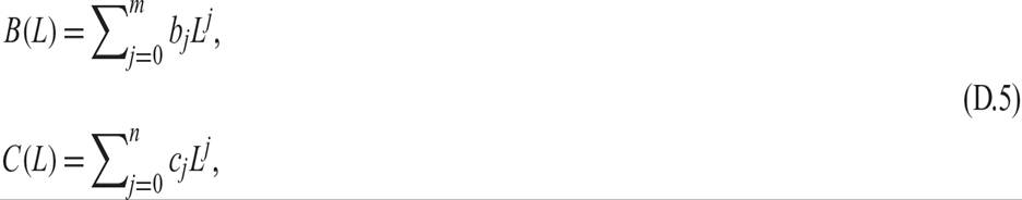
and b_j and c_j are constants. The combination of (D.4) and (D.5) imposes a more economical and restrictive form on a_j, without serious loss of generality.

A special case of (D.4) and (D.5) is the so-called geometric polynomial, which takes the form

From the properties of geometric progressions, the geometric polynomial can be expanded in two ways:

The expansion (D.7) is used when |λ| < 1, and the expansion (D.8) when |λ| > 1.

If we multiply the geometric polynomial (D.6) by some variable x_t, we get

With the expansion (D.7) for A(L) we get

If |λ| < 1, and is a finite sequence of real numbers, then (D.10) defines a finite sequence of real numbers as well.

In contrast, we have the alternative expansion of (D.9). Using (D.8), we get

If |λ| > 1, and is a finite sequence of real numbers, then (D.11) defines a finite sequence of real numbers as well, because we have |λ⁻¹| < 1.

In economics, because we usually seek convergence to some equilibrium, we seek the analysis of finite sequences. Thus, we select the backward expansion when |λ| < 1, and the forward expansion when |λ| > 1.

A difference equation (or recurrence relation) equates a polynomial in the various iterates of a variable—that is, in the values of the elements of a sequence—to zero.

An nth-order linear difference equation with constant coefficients takes the form

where a_j, j = 0, 1, 2, …, n and b are constant coefficients.

By equating the right-hand side of the geometric polynomial (D.10) to zero, we get

This is an example of an infinite-order linear difference equation.

D.2 First-Order Linear Difference Equations

Let us first consider the first-order linear difference equation with constant coefficients:

Using lag operators, (D.14) can be written as

Dividing both sides of (D.15) by (1 − bL) and adding cb^t, we get

where c is an arbitrary constant.

Hence, if we multiply (D.16) by (1 − bL), we get back (D.15). Equation (D.16) determines the general solution of the linear first-order difference equation (D.14).

To find a particular solution, we must determine c. Assume that in period t = 0, x had the value x₀. From (D.16), it follows that

Thus, the particular solution of (D.14) is given by

If the boundary condition is such that x₀ = a/(1 − b), then (D.18) implies that

Thus, a/(1 −b) can be seen as an equilibrium value. If x = a/(1 −b), then x tends to stay at this level.

In addition, x₀ if |b| < 1, (D.18) implies that for any x₀, we have

Equation (D.19) implies that the difference equation is stable, because x tends to approach its equilibrium value over time from any initial condition. In this case, the equilibrium value is a stable node.

If |b| > 1, the only path that leads to the equilibrium value is the immediate jump of x to the equilibrium value a/(1 − b). This solution requires

The equilibrium value in this case is a saddle point.

D.3 Second-Order Linear Difference Equations

We next turn to the second-order linear difference equation with constant coefficients, of the form

Using the lag operator, (D.20) can be written as

Equation (D.21) can be expressed as

where

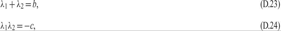
and λ₁ and λ₂ are the two roots of the second-order linear difference equation (D.20).

There are three possible cases, depending on the discriminant of the characteristic equa-tion of (D.20).

Case 1 b² > −4c The discriminant is positive, and the roots are real and distinct, taking the form

From (D.22), the general solution of (D.20) takes the form

where d₁ and d₂ are two arbitrary constants. To determine the arbitrary constants, one needs two boundary conditions, depending on the values of the two roots.

As in the case of a first-order difference equation, a/(1 −b−c) can be seen as the equili-brium value of x.

We have convergence to the equilibrium value if |λ₁| < 1 and |λ₂| < 1. In this case, the equilibrium value will be a stable node, and to determine the two arbitrary constants, d₁ and d₂, we need two initial conditions x₁, x₂ ≠0.

If the two roots lie on either side of unity (i.e., if |λ₁| < 1 and |λ₂| > 1), then the equilibrium value will be a saddle point. In this case, to determine the two arbitrary constants d₁ and d₂, we need one initial and one final condition. The final condition can be none other than the equilibrium value. As a result, we shall have convergence to the equilibrium value only if d₁≠0 and d₂ = 0.

If both roots are greater than unity (i.e., if |λ₁| > 1 and |λ₂| > 1), then the only solution is the immediate jump of x to the equilibrium value a/(1 − b − c). This solution requires d₁ = 0, d₂ = 0, and x_t = a/(1 − b − c) for all t.

Case 2 b² = −4c The discriminant is equal to zero, and we have two equal real roots of the form

The general solution takes the form

If |λ| < 1, to determine the two arbitrary constants d₁ and d₂, we need two initial conditions.

If λ is greater than unity in absolute value (i.e., if |λ| > 1), then the only solution is the immediate jump of x to the equilibrium value a/(1 − b − c). This solution requires d₁ = 0, d₂ = 0, and x_t = a/(1 − b − c) for all t.

Case 3 b² < −4c The discriminant is negative, and we have two complex roots, which take the form of a pair of complex conjugates:

where , and .

Using De Moivre’s theorem and the Pythagorean theorem the solution takes the form

where R and θ are defined by

and

This solution will produce oscillations of a periodic nature. The oscillations will be dampened if and only if |c| < 1. In such a case, there will be cyclical convergence to the equilibrium value. In the case |c| < 1, there will be continuous oscillations of a constant periodicity. And if |c| > 1, there will be divergent oscillations, unless x jumps immediately to its equilibrium value.

D.4 A Pair of First-Order Linear Difference Equations

We next turn to a second-order system of two linear first-order difference equations. The system is described by

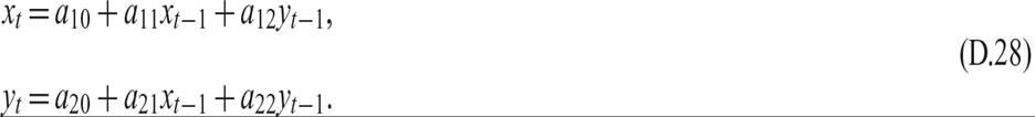
As in the case of a system of two first-order differential equations, the first method of solving this system is the substitution method. We can use the second equation to substitute for y_t−1 in the first equation, and thus obtain a second-order difference equation in x:

where a = (a₁₀(1 − a₂₂) + a₁₂a₂₀), b = a₁₁ + a₂₂, and c = −(a₁₁a₂₂ − a₁₂a₂₁).

Equation (D.29) has the same form as (D.20) and can be solved as an ordinary second-order linear difference equation with constant coefficients. Making use of the lag operator, the homogeneous equation corresponding to (D.29) can be written as

The two roots of the polynomial in the lag operator must satisfy the characteristic equation

By going through the alternative substitutions, a similar second-order difference equation can be obtained for the second variable y_t.

Alternatively, one can rewrite the system (D.28) in matrix form as

The homogeneous system corresponding to (D.32), with a₁₀ = a₂₀ = 0, takes the form

Using the lag operator L, (D.33) can be rewritten as

For (D.33) to have a solution, the matrix in the lag operator must be singular. Therefore, its determinant must be equal to zero. Thus, for a solution to exist, we must have

This condition implies a polynomial in the lag operator with characteristic equation

which is identical to (D.31), the characteristic equation of the second-order difference equation (D.29), and will of course give the same solution for the two roots.

However, even this solution method becomes unwieldy for higher-order systems when there are more than two variables. It is thus desirable to investigate other solution methods. To do so, it is worth generalizing the system to one of n first-order linear difference equations.

D.5 A System of n First-Order Linear Difference Equations

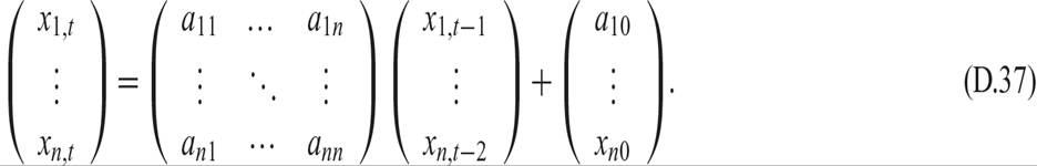
Let us consider the following system of n first-order difference equations. Such systems arise quite often in dynamic macroeconomics:

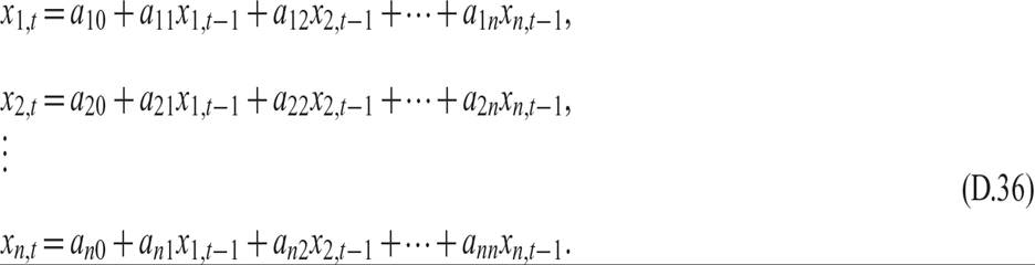
In matrix form, the system (D.36) can be written as

By defining the vector of xs as x, the matrix of multiplicative parameters as A, and the vector of the constants as a₀, the system can be written as

If a_ij = 0 for i≠j in the system (D.37), then the n equations are uncoupled, and the system can be solved as n independent first-order linear difference equations with solutions

where x_{i, 0} is a boundary value for x_i.

Thus, if we could transform the system (D.37) into one with a coefficient matrix that is diagonal, we could easily calculate the solution. The question is how to transform the system into one with a diagonal coefficient matrix.

We know from the properties of matrices that the coefficient matrix A can be transformed as

where J is a diagonal matrix with the eigenvalues of A on its diagonal, and P is a matrix consisting of the corresponding (right) eigenvectors. Equation (D.40) implies that

We can use these properties to rewrite the system (D.38) as

Multiplying both sides of (D.42) by P⁻¹, we get

Defining a new vector of variables X_t = P⁻¹x_t, and a new vector of constants A₀ = P⁻¹a₀, we can rewrite (D.38) as

Thus, by using the matrix consisting of the eigenvectors of the original coefficient matrix A to define new variables and new constants, we can transform the original coupled system of difference equations to a system of decoupled difference equations in the newly defined variables, as in the case of differential equations. The decoupled system can be solved for each of the transformed variables in X. We can then find the solutions for the original vector of variables by using the reverse transformation

By using the diagonal matrix of the eigenvalues of A and the matrix of the corresponding (right) eigenvectors, we can solve the system of n first-order linear difference equations (D.36). The solution method is similar in spirit to the one for a system of n first-order differential equations discussed in appendix C.

1. This appendix is meant as a review and is not a full and rigorous analysis of difference equations. For more complete treatments, the student is referred to comprehensive textbooks on mathematics for economists, such as Chiang [1974], Simon and Blume [1994], or Klein [2013]. A very good treatment of difference equations can be found in Sargent [1987].