Appendix C: Ordinary Differential Equations

In this mathematical appendix, we review solution methods of linear differential equations and systems of linear differential equations. Knowledge of the properties of differential equations is indispensable for analyzing problems in continuous time in dynamic macroeconomics.

We start with some definitions, and then proceed to examine solution methods of first-and second-order differential equations with both constant and variable coefficients. We finally briefly discuss the generalization of the solution methods to a system of n first-order differential equations.¹

C.1 Definitions

A differential equation is a mathematical equation derived from an unknown function of one or more variables, which connects the function itself and its derivatives of various degrees.

The solution of a simple equation (or a system of equations) is a constant or a set of constants that satisfy these equations. In contrast, the solution of a differential equation (or a system of differential equations) is a function, or a set of functions that, along with their derivatives, satisfy the differential equation or the system of differential equations. The equations we shall consider are all functions of time t, which is assumed to be a continuous variable defined on the set of real numbers ℝ.

For example, the solution to the differential equation

is a function y(t), the first derivative of which with respect to time is equal to a. The general solution to this differential equation is the function

where c is an arbitrary constant.

A particular solution can be found by using a boundary condition. For example, if we know that at t = 0, y is equal to y₀ (known as the boundary value), then a particular solution of (C.2) is given by setting c to c = y₀.

Another example is the differential equation

whose solution is

where b and c are two arbitrary constants.

A solution of a differential equation is a function y(t), which, along with its derivatives, satisfies the differential equation. A general solution is the full set of solutions of a differential equation. A particular solution requires the determination of the arbitrary constant or constants of integration.

Differential equations are classified by their order, which is none other than the order of the highest derivative that appears in the equation. For example, (C.1) is a first-order differential equation, whereas (C.3) is a second-order differential equation.

A differential equation is linear if the unknown function y(t) and its derivatives are linear. Otherwise it is nonlinear.

A differential equation can be solved by a method known as separation of variables if it can be written as a term that contains a function of only y, equated to a term that contains a function only of t. For example, the equation

can be written as

The variables are separated, and the solution is

where c is an arbitrary constant.

Finally, a differential equation

which is equivalent to

is called exact if there is a function U(t, y) that satisfies

Thus, a differential equation is exact if it constitutes exactly the total differential of a function.

C.2 First-Order Linear Differential Equations

First-order linear differential equations are categorized as equations with constant coefficients, or those with variable coefficients.

C.2.1 Constant Coefficients

A first-order linear differential equation with constant coefficients takes the form

where a and b are given constants. To find the function y(t) that satisfies (C.11), note that

If the differential equation (C.11) is multiplied by e^at, its left-hand side is an exact differential equation) (i.e., the total differential of a function with respect to t). The function e^at is called the integrating factor. Multiplying both sides of (C. 12) by dt, we get

where c is the constant of integration. Multiplying both sides of this expression by e^−at, we get

as the family of functions that satisfy the differential equation (C.11). This family is called the general solution of (C.11).

To determine the constant of integration c, we need to know the value of the function at some point in time. For example, if we know that at time t = 0, y(0) = y₀, then

which implies

The general solution of the differential equation (C.11) that satisfies y(0) = y₀ is then given by

In conclusion, to solve a linear first-order differential equation with constant coefficients, multiply it by the integrating factor and integrate it.

C.2.2 Variable Right-Hand Side

If the right-hand side of (C.11) is not constant but a known function of time, the solution method is similar. We multiply by the integrating factor and take the integral.

For example, for the differential equation

multiplying by the integrating factor and separating the variables results in

Taking the integral of both sides of (C.16) yields

Dividing both sides by the integrating factor, we get the solution

Equation (C.18) is the family of functions satisfying (C.15). The unknown constant c can again be determined by a boundary condition.

C.2.3 Variable Coefficients

The general form of a first-order linear differential equation is

where a(t) and b(t) are known functions, and we seek the function y(t). The function b(t) is often called a forcing term and is considered exogenous. The integrating factor in this case is e^{∫ a(t)dt}, because

Thus, multiplying (C.19) by this integrating factor and taking the integral, we get

Dividing (C.21) by the integrating factor, we finally get

where c is the constant of integration.

Note that it is not advisable to apply the solution (C.22) to any equation. It is simpler in many cases to multiply by the integrating factor and take the integral.

C.2.4 Homogeneous and Nonhomogeneous Differential Equations

If b = 0 in (C.11), the differential equation to be solved is called homogeneous. Otherwise, it is called nonhomogeneous.

The general solution of a differential equation consists of the sum of the general solution to the relevant homogeneous differential equation (i.e., setting b = 0 and solving, and then adding to this solution a particular solution of the general equation (C.11).

For example, the homogeneous equation derived from (C.11) is

The general solution of (C.23) is

A particular solution (setting, for example, ) is

Consequently, the general solution of the nonhomogeneous differential equation (C.11) is the sum of (C.24) and (C.25), that is, the general solution of the relevant homogeneous differential equation (sometimes called the complementary function) plus the particular solution for a constant y (otherwise known as the particular integral). The general solution is thus given by

This methodology is not generally necessary for solving first-order linear differential equations, but it becomes very useful for differential equations of order higher than one or for systems of first-order linear differential equations.

C.2.5 Convergence and Stability of First-Order Differential Equations

In many economic applications, we are interested in the behavior of the solution of a differential equation as the independent variable, usually time, tends to infinity. The value to which the solution converges is referred to as a stationary state, or steady state, or equilibrium state.

For example, from (C.13), which is the general solution of (C.11), for a > 0, we get

The particular integral of the differential equation (C.11) can therefore be interpreted economically as the equilibrium state (or the steady state), which is the state toward which the variable y converges as time goes to infinity. This equilibrium is called a stable node. It is a stable equilibrium if y is a predetermined variable and only changes gradually, as postulated by the law of motion (C.26).

Assume now that a < 0. In this case, if the boundary condition y₀ is different from the steady value y, then y(t) (as determined by (C.26)) moves to plus or minus infinity, farther and farther away from the steady state. The only case in which this does not happen is when the boundary condition y₀ is equal to the steady state value y = b/a. Then y remains constant at y. However, this is an unstable equilibrium, called a saddle point. There is only one adjustment path that leads to it and this is for y to jump immediately to the steady state. If y is a non-predetermined variable (for example, a financial variable or any variable that can change abruptly and not gradually), then it can jump immediately to its steady state value.

C.3 Second-Order Linear Differential Equations

A second-order linear differential equation has the form

where a(t), b(t), and h(t) are known functions, and what is sought is the function y(t). The forcing term in this case is the function h(t). Equation (C.27) is referred to as the complete equation and is nonhomogeneous. Related to (C.27) is a homogeneous differential equation in which h(t) = 0:

which is called the reduced equation. The complete equation is nonhomogeneous, whereas the reduced equation is homogeneous. The reduced equation is of interest because of the following two theorems.

Theorem 1 The general solution of the complete equation (C.27) is the sum of any particular solution of the complete equation and the general solution of the reduced equation (C.28).

Theorem 2 Any solution y(t) of the reduced equation (C.28) on t₀ ≤ t ≤ t₁ can be expressed as a linear combination, y(t) = c₁y₁(t) + c₂y₂(t), t₀ ≤ t ≤ t₁, of any two particular solutions y₁, y₂ that are linearly independent.

C.3.1 Homogeneous Equations with Constant Coefficients

We first examine the differential equation (C.27), with constant coefficients, that is, a(t) = a, b(t) = b. Assume that h(t) = 0. The differential equation then takes the form

Inspired by the general solution of the first-order linear differential equation with constant coefficients, let us try the general solution

with unknown constants c and r. This solution method is called the method of undetermined coefficients. This solution implies that

Substituting these expressions in (C.29), we get

For a nonzero c, our trial solution satisfies (C.30) only if r is a root of the quadratic equation

Equation (C.31) is called the characteristic equation of (C.29). It has two roots:

We distinguish three cases, depending on the value of the discriminant a² − 4b of the characteristic equation (C.31).

Case 1 a² > 4b The discriminant is positive, and the roots are real and distinct. The general solution of (C.29) takes the form

where r₁, r₂ are the roots of the characteristic equation (C.31), and c₁, c₂ are arbitrary constants.

Case 2 a² < 4b The discriminant is negative, and the roots are a pair of complex conjugates:

where , and . The general solution in this case is

where k₁, k₂ are arbitrary constants.

Case 3 a² = 4b The discriminant is equal to zero, and the two roots are the same and equal to − a/2. One can show that the general solution of (C.29) in this case takes the form

where r = −a/2 is the double root of the characteristic equation (C.31), and c₁, c₂ are arbitrary constants.

C.3.2 Nonhomogeneous Equations with Constant Coefficients

We have already derived the solution of any homogeneous second-order linear differential equation with constant coefficients. To find the solution of a nonhomogeneous equation, we need a particular solution of the complete equation. If the complete equation is of the form

then a particular solution is the constant function

The full solution is thus the sum of the general solution to the homogeneous equation plus the particular solution to the complete equation.

For differential equations with variable coefficients, more advanced methods, such as the method of variation of parameters, can be utilized for their solution.

C.4 A Pair of First-Order Linear Differential Equations

We next examine a case with extensive applications in macroeconomics: a pair of first-order linear differential equations of the form

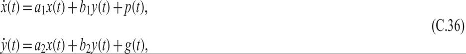
where a₁, a₂, b₁, b₂ are given constants, and p(t), g(t) are given functions. The solution of the system of differential equations (C.36) will be two functions x(t) and y(t) that satisfy both differential equations.

The homogeneous system that corresponds to (C.36) is given by

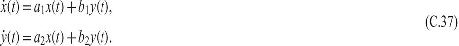
C.4.1 The Method of Substitution

One solution method is the method of substitution. Substituting y(t) and its derivatives in the equation determining x(t), we end up with a second-order linear differential equation that contains only x(t) and its derivatives:

Equation (C.38) is a linear homogeneous second-order differential equation. It can be solved using the method of undetermined coefficients. Its characteristic equation is given by

If the roots of (C.39) are real and distinct, the solution of (C.38) is given by

Solving the first equation of (C.37) with respect to y(t), we get

Substituting the solution (C.40) for x(t) and its first derivative, we get

Consequently, the solution of the system (C.37) consists of equations (C.40) and (C.41), if the roots of (C.39) are real and distinct. We can solve the system in an analogous way if we have complex or repeated roots.

However, there is a second and more direct solution method of the homogeneous system (C.37). This method also generalizes to higher-order systems of differential equations.

C.4.2 The Method of Eigenvalues

Our experience with first-order differential equation suggests that we use the pair of equations

alt=pg676-1.png>

as particular solutions for (C.37). Here A, B, and r are undetermined coefficients. Substituting these solutions in (C.37), we get

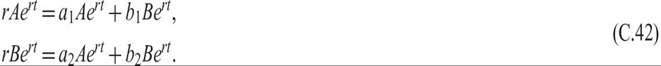
Dividing both equations by e^rt, we can rewrite the system (C.42) in matrix form:

For (C.43) to hold, the determinant of the matrix of coefficients must be zero:

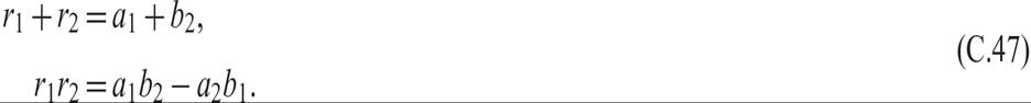
Calculating the determinant, we get a quadratic equation in r:

Equation (C.45) is the characteristic equation of the system (C.37). Equation (C.45) is identical to (C.39), the equation we ended up with when using the method of substitution. The solutions of the characteristic equation (C.45) are called the eigenvalues of the matrix of coefficients:

The two roots are given by

For future use, note that

If the roots are real, and r₁≠r₂, then the general solution of the homogeneous system (C.37) is given by

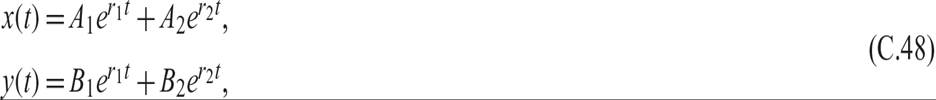
where A₁, A₂ are determined by boundary conditions; the roots are determined by (C.46); and B₁, B₂ are determined by (C.42) as

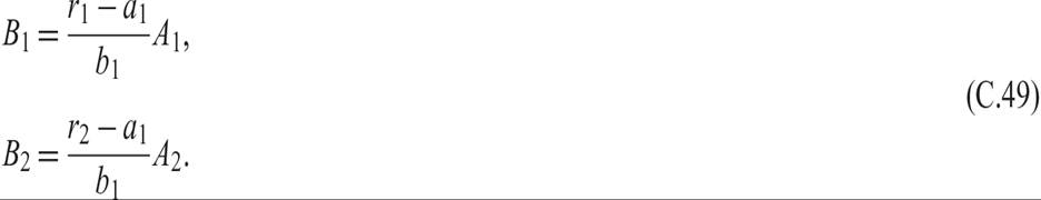
The solution is identical to (C.40) and (C.41). In the case of complex or repeated roots, the solution is analogous.

Having found the general solution to the homogeneous system (C.37), it remains to find a particular solution of (C.36), using, for example, the method of variation of parameters.

For the special case where p and g are constants, a special solution with constant x and y can be found by solving the system of equations

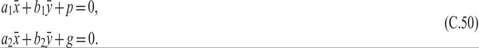
Expressing (C.50) in matrix form and solving for and y, we get

The solution is then given by

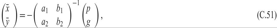
where and y can be regarded as steady state, or equilibrium points. Whether the system converges globally to equilibrium depends on whether both roots are real and smaller than zero. In this case, the equilibrium is a fixed node. If both variables are predetermined, this is a stable equilibrium.

If we have a positive and a negative root, the equilibrium is called a saddle point. There is only one unique path that leads to this equilibrium, and this path is called the saddle path. The economy will converge to equilibrium if one variable is predetermined and the other not predetermined. The non-predetermined variable will jump to the unique adjustment path leading to equilibrium. Technically, the negative root corresponds to the predetermined variable (for which we solve backward), and the positive root corresponds to the non-predetermined variable (for which we solve forward).

Thus, a system with one predetermined and one non-predetermined variable has an equilibrium (a saddle point) if the matrix of coefficients has one positive and one negative eigenvalue.

C.5 A System of n First-Order Linear Differential Equations

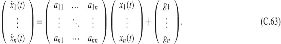
Finally, we turn to a more general case with extensive applications in macroeconomics: a system of n first-order linear differential equations of the form

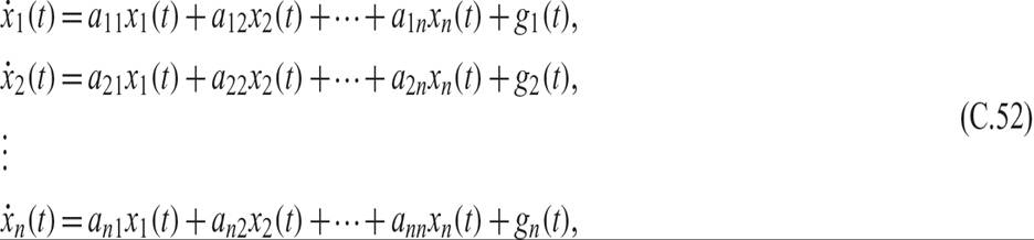
where x₁, x₂, …, x_n, a_ij for i, j = 1, 2, …, n are given constant parameters, and g₁, g₂, …, g_n are exogenous forcing functions of time.

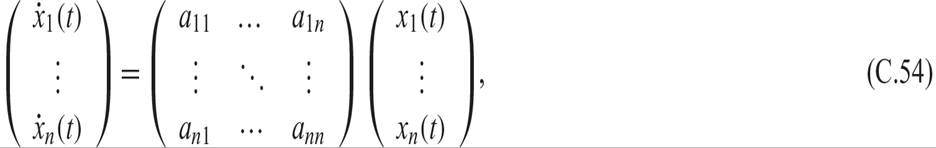
In matrix form, this system can be written as

or

where bold letters denote vectors and matrices; A is the square n ? n coefficient matrix, which is assumed to be nonsingular.

C.5.1 Eigenvalues and Eigenvectors

Before we proceed to discuss the solution of the system of differential equations (C.52), it is worth delving a little more into linear algebra, and in particular, into the concepts of eigenvalues and eigenvectors.

Let A be a square matrix, like the one multiplying the x vector in the right-hand side of (C.53). An eigenvalue of A is a number ρ, which when subtracted from each of the diagonal elements of A converts A into a singular (i.e., noninvertible) matrix. Subtracting a scalar ρ from each of the diagonal elements of A is equivalent to subtracting from A ρ times the identity matrix I. Therefore, ρ is an eigenvalue of A if and only if A − ρ I is singular.

Because a matrix is singular if its determinant is equal to zero, ρ is an eigenvalue of A if and only if

For an n ? n matrix A, the determinant of A − ρ I is an nth-order polynomial in ρ, called the characteristic polynomial of A. An nth-order polynomial has at most n roots. Therefore, an n ? n square matrix has at most n eigenvalues.

It follows from the above that the diagonal entries of a diagonal matrix D are eigenvalues of D, and that a square matrix A is singular if and only if 0 is an eigenvalue of A.

Recall from elementary linear algebra that a square matrix B is nonsingular if and only if the only solution of Bx = 0 is x = 0. Conversely, B is singular if and only if the system Bx = 0 has a nonzero solution.

The fact that A − ρ I is singular when ρ is an eigenvalue of A means that the system of equations (A − ρ I)v = 0 has a solution other than v = 0.

When ρ is an eigenvalue of A, a nonzero vector v such that (A − ρ I)v = 0, is called a (right) eigenvector of A, corresponding to the eigenvalue ρ.

Thus, eigenvectors are nonzero vectors v that satisfy

These three statements are equivalent.

C.5.2 Solving the nth-Order System of Linear Differential Equations

Let us now turn to the solution of the nth-order system of linear differential equations represented by (C.52). The general solution of the nonhomogeneous system of differential equations (C.52) will be the sum of the general solution of the relevant homogeneous system of differential equations plus the particular solution for constant xs.

We shall concentrate on the solution of the homogeneous system

or simply, , where x is the column vector on the right-hand side of (C.54).

Assume first that A is a diagonal matrix, for which a_ij = 0 for i≠j. Then (C.54) becomes a system of n independent self-contained equations of the form

We thus have a system of independent first-order linear differential equations that can be solved one by one:

If the off-diagonal elements a_ij differ from zero, so that the equations are linked to each other, then we can use the eigenvalues and eigenvectors of the coefficient matrix of (C.54) to transform it to a system of n (or fewer) independent equations. We can use the eigenvalues and eigenvectors of A to transform the system to a system that has a diagonal coefficient matrix.

Let us assume that A has n distinct real eigenvalues ρ₁, ρ₂, …, ρ_n, with corresponding eigenvectors v₁, v₂, …, v_n. It then follows from the definition of eigenvalues and eigenvectors that

Let P be the n ? n matrix whose columns are these n eigenvectors. Thus P is defined as

The system of equations (C.55) can thus be written as

where

Because eigenvectors for distinct eigenvalues are linearly independent, P is nonsingular and therefore invertible. We can write

Thus, we can use (C.56) to transform the system (C.52), defined in the variables x, to a system in the variables y = P⁻¹x, which means that x = Py. It follows that

Because J is a diagonal matrix, the solution of the system (C.59) can be obtained very easily as the vector of solutions to each variable y_i:

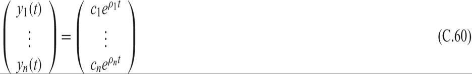
Finally, we can use the transformation x = Py to return to the original variables x₁, …, x_n:

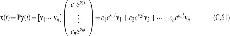
Thus, under the assumption that the n ? n matrix A has n distinct real eigenvalues ρ₁, ρ₂, …, ρ_n, with corresponding eigenvectors v₁, v₂, …, v_n, the general solution of the homogeneous linear system (C.52) is given by

The solution in the cases of complex eigenvalues or multiple eigenvalues without enough eigenvectors is analogous to the solution of the second-order homogeneous system analyzed in section C.4.

Steady states and stability conditions are defined in an analogous way to those for first-and second-order differential equations. Assuming that the vector of gs consists of constants, one gets the nonhomogeneous system:

The steady state, if it exists, can be derived by setting the change in the xs equal to zero. A steady state exists if A is nonsingular and is given by

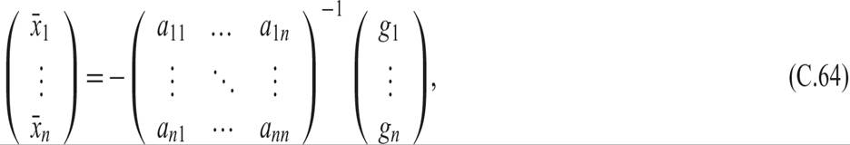
where _i denotes the steady state value of x_i. These values can be regarded as equilibrium points. If the x_is are predetermined variables, for the system to converge to equilibrium, all eigenvalues must be less than zero. In this case, the equilibrium is a fixed node. When the x_is consist of p predetermined and q non-predetermined variables, where p + q = n, the equilibrium (if it exists) is a saddle point. For the system to converge to equilibrium, there must be p negative eigenvalues and q positive eigenvalues. The negative eigenvalues correspond to the predetermined variables, which are solved for backward, and the positive eigenvalues correspond to the non-predetermined variables which are solved for forward.

Thus, a system with p predetermined and q non-predetermined variables has a stable equilibrium (a saddle vector) if the matrix of coefficients has p negative and q positive eigenvalues. The adjustment path is unique and is called a saddle path.

1. This appendix is a review and a toolkit, designed to help students refresh their knowledge. It is not a complete mathematical treatment. For fuller and more rigorous mathematical treatments of ordinary differential equations, see Boyce and DiPrima [1977] or any comprehensive textbook of mathematics for economists, such as Chiang [1974], Simon and Blume [1994], or Klein [2013].