Appendix B: Linear Models and Linear Algebra

In this appendix, we discuss the solution of linear economic models and introduce the basic elements of linear algebra. Linear algebra is the branch of mathematics that analyses vector spaces and linear mappings between such spaces.

Because linear algebra is such a well-developed branch of mathematics, nonlinear models are sometimes approximated by linear models. Combined with calculus, linear algebra also facilitates the solution of linear systems of differential and difference equations. This appendix provides a review of the main elements of linear algebra.¹

B.1 Linear Models

Consider the following system of linear equations, where y_i, i = 1, 2, …, n, denotes an endogenous variable; x_j, j = 1, 2, …, m, denotes an exogenous variable; and a_ik and b_ij denote constant parameters, with k = 1, 2, …, n:

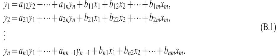
The system of equations (B.1) is an example of a linear economic model, with n endogenous variables, and m exogenous variables determined outside the model. Because it contains n equations in n unknowns (the n endogenous variables), it could in principle be solved for the values of the endogenous variables as functions of the exogenous variables.

Under what conditions does this model possess a solution? Is the solution unique? How do the exogenous variables affect each endogenous variable?

To answer these types of questions and to be able to derive the solution of the model, we need to use some concepts of linear algebra. The model in (B.1) can be rewritten in matrix form.

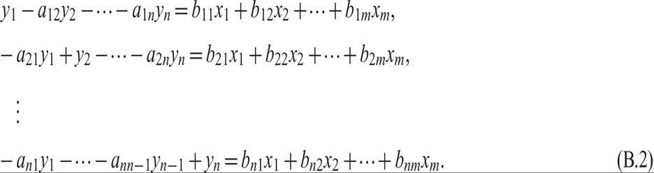
The system (B.2) can be represented in matrix form:

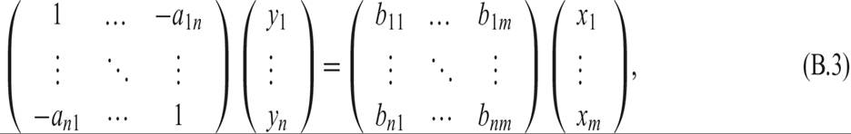
where the rectangular arrays of the a_iks and the b_ijs are matrices of coefficients, and the vertical arrays of the endogenous and exogenous variables are vectors of variables.

B.2 Elements of Linear Algebra

A table with n rows and m columns, such as the one containing the b_ijs in equation (B.3) is called an n?m matrix. The elements of the matrix can be either scalars or variables. For example, b₁₁ is the scalar in the first row and the first column of the matrix containing the b_ijs.

A matrix with the same number of rows and columns, such as the matrix containing the a_iks in (B.3), is called a square matrix. In this case, it is an n ? n square matrix.

A matrix with one column, such as the one containing the endogenous and exogenous variables, is called a vector.

The system of equations (B.1) in matrix form, as in (B.3), can be represented more compactly as

where A denotes the n ? n square matrix of the coefficients of the endogenous variables in (B.3), B denotes the n ? m matrix of the coefficients of the exogenous variables in (B.3), and y and x denote the vectors of the endogenous and the exogenous variables, respectively.

One can perform matrix algebra on matrices and thus analyze systems of equations in matrix form.

B.2.1 Matrix Addition, Subtraction, and Multiplication

One common matrix operation is scalar multiplication. If B is an n ? m matrix, then multiplying B by a scalar λ entails multiplying each element of the matrix by λ.

A second type of operation is matrix addition and matrix subtraction. For these operations to be meaningful, the matrices must be of the same dimension. Thus, if B and C are two n ? m matrices, we can define a new matrix D = B + C, or an new matrix E = B − C. The elements of D are the sum of the corresponding elements of B and C, and the elements of E are the difference between the corresponding elements of B and C. Thus, element d_ij = b_ij + c_ij in the D matrix, and element e_ij = b_ij − c_ij in the E matrix.

A third operation, matrix multiplication, requires two compatible matrices as well. To multiply two matrices B and C, the number of columns of matrix B must be equal to the number of rows of matrix C. Assume that B is an m ? n matrix, and C is an n ? p matrix. Then the product of the two matrices is the m ? p matrix D = BC, whose element d_ij is the inner product of the ith row of matrix B with the jth column of matrix C, defined as d_ij = ∑ _k=1ⁿb_ikc_kj.

These matrix operations also apply to vectors.

It is straightforward to verify that the products Ay and Bx in (B.4) exist, because the matrices multiplied are indeed compatible. Both Ay and Bx turn out to be n ? 1 vectors.

Another useful matrix operation is transposition. The transpose of matrix is a new matrix whose rows are the columns of the original matrix, and its columns are the rows of the original matrix. Thus, if B is an n?m matrix, its transpose B^T, or B′ is an m ? n matrix.

B.2.2 The Inverse of a Square Matrix

The final, and more involved operation involving matrices is matrix inversion. This is the equivalent of division for scalars, and it only applies to square matrices. To be able to divide by a matrix A, we must define the inverse of A.

Consider an n x n square matrix A, defined as

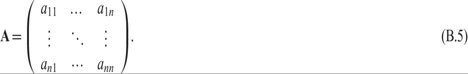
The main diagonal of this matrix consists of all the elements a_ii, i = 1, 2, …, n. The main diagonal is also the first diagonal of the matrix. Diagonals are defined by the n elements on the diagonal of the matrix from left to right, as we go down the rows. The main diagonal is given by (a₁₁, a₂₂, …, a_nn). The second diagonal is given by (a₁₂, a₂₃, …, a_n−1n, a_n1). The nth diagonal is given by (a_1n, a₂₁, …, a_n−1n). The second diagonal is the main diagonal of a matrix in which the first column has been moved to the end, and the second column has become the first column. The ith diagonal is the main diagonal of a matrix in which the first i − 1 columns have been moved en block to the end, and the ith column has become first.

The antidiagonals of this matrix are defined as the n elements on the diagonals of the matrix from right to left, as we go down the rows. The main antidiagonal is given by (a_1n, a_2n−1, …, a_n1). The other antidiagonals are defined analogously. The ith antidiagonal is the main antidiagonal of a matrix in which the first i − 1 columns have been moved en block to the end, and the ith column has become the first column.

To define the diagonals and antidiagonals, it is sometimes useful to consider the augmented matrix A|A, defined by

It is quite easy to define the n full diagonals and antidiagonals of A using this augmented matrix.

A special square matrix is the identity matrix. This is denoted by I, and is a matrix that has 1s across its main diagonal, and 0s elsewhere:

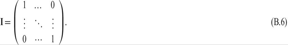
The identity matrix plays the role of unity in matrix algebra.

for any square matrix A.

From (B.7) it follows that, if the inverse A⁻¹ of matrix A exists, then it should satisfy

For the inverse of A to exist, A must be a full rank matrix. For the moment, it suffices to say that a full rank matrix’s rows or columns must be linearly independent. For a square matrix to be full rank, its determinant must be nonzero.

The determinant of an n ? n square matrix A is denoted and defined by the following formula:

where |A_ij| is the minor of element a_ij, defined as the determinant of the matrix that results when row i and column j are deleted from matrix A. Hence, the determinant is defined in terms of the elements of row i and the minors of these elements, which are also determinants.

The term

is called the cofactor of the element a_ij. Hence, the determinant is also defined in terms of the elements in the ith row of a matrix, multiplied by their cofactors.

If one were to choose row 1 for i, then the determinant is defined by

For example, for a 2 ? 2 matrix, the determinant is defined as

For a 3 ? 3 matrix, it is defined as

This expression can be expanded as

For higher-order matrices, the calculation is even more complicated, although the principle is quite straightforward.

Armed with these elements from linear algebra, the solution of the linear economic model (B.4) is in principle straightforward. If the inverse of the square coefficient matrix A exists, then the solution takes the form

Equation (B.10) expresses the endogenous variables y_i, i = 1, 2, …, n, as functions of the exogenous variables x_j, j = 1, 2, …, m.

B.3 An Example with Two Endogenous Variables

In this section, let us apply linear algebra to a model with two endogenous and two exogenous variables. The model in matrix form is given by

The A matrix is given by

The determinant of the A matrix is given by

Thus, A will be full rank if and only if a₁₂a₂₁≠1.

The inverse of A can be calculated by a number of methods.

B.3.1 Cramer’s Rule

The first method is Cramer’s rule. The inverse is given by

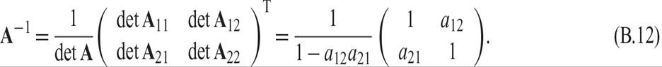
The matrix premultiplied by the inverse of the determinant of A is called the adjoint matrix of A, and it is the transpose of the matrix of cofactors of A. A cofactor of an element a_ij of a square matrix A is the determinant of the matrix A_ij that results if we eliminate the row and the column containing a_ij and multiply by −1^i+j.

B.3.2 The Augmented Matrix and Gauss-Jordan Elimination

A second—and computationally more efficient—method for inverting larger matrices is the augmented matrix method. This method uses Gauss-Jordan elimination to transform the augmented matrix [A|I] into the equivalent augmented matrix [I|A⁻¹]. This is done by transforming the system’s augmented matrix into reduced row-echelon form by means of row operations.

The augmented matrix of A is given by

Through successive row operations, such as replacing row 2 by the sum of row 2 and the product of a₂₁ and row 1, then dividing the resulting row 2 by 1 − a₁₂a₂₁, and finally replacing row 1 by the original row 1 minus the product of a₁₂ and row 2 of the previous step, we end up with

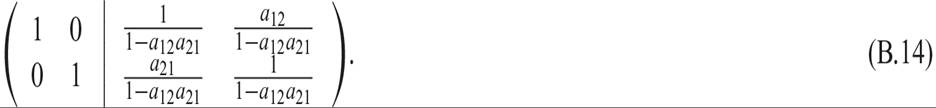
The matrix on the right-hand side of the transformed augmented matrix is the inverse of A.

B.3.3 Diagonalization, Eigenvalues, and Eigenvectors

A third method of solving the system (i.e., investing the matrix) is through the diagonalization of A, using the eigenvalues and the eigenvectors of A. We postpone the discussion of this method until we discuss the solution of systems of differential equations.

B.3.4 Solving a System with Two Endogenous and Two Exogenous Variables

We can apply these matrix methods to the solution of the system (B.10) with two endogenous and two exogenous variables. This is a system of two equations with two unknowns. The ys, can in principle be solved as functions of the exogenous variables, the xs.

As this is a low-dimensional system, we can first attempt to solve it through a nonmatrix method, such as the method of substitution. This will allow us to check the results of matrix methods, such as Cramer’s rule and Gauss-Jordan elimination.

The system in (B.10) can be written in nonmatrix form as a system in the two unknown ys. It takes the form

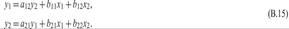
The system can be solved by the method of substitution. Using the second equation in (B.15) to substitute for y₂ in the first equation, the solution for y₁ takes the form

Note that a₁₂a₂₁≠1, for y₁ to have a finite solution. Otherwise, y₁ is not defined. This is the same as the condition that the determinant of the matrix of coefficients of the ys must be nonzero.

Substituting (B.16) for y₁ in the second equation of (B.15), the solution for y₂ takes the form

The system of solved equations (B.16) and (B.17) is called the reduced form of the original structural form of the system (B.15). There are finite solutions for y₁ and y₂ if and only if a₁₂a₂₁≠1.

By applying Cramer’s rule to the same system in matrix form, the system solution of (B.10) is given by

Carrying out the matrix multiplications, we get

Equation (B.18) is identical to the reduced form system (B.16)–(B.17).

It is straightforward to confirm that the same solution applies if one uses the Gauss-Jordan elimination method to find the inverse of the matrix of coefficients of the endogenous variables A.

1. This review is neither a complete nor a mathematically rigorous treatment but is adequate for the purposes of this text. For fuller and more rigorous treatments of linear algebra suitable for economists, consult a comprehensive text of mathematics for economists, such as Chiang [1974], Simon and Blume [1994], or Klein [2013].