Appendix A: Variables, Functions, and Optimization

In this appendix, we review some basic mathematical concepts and techniques required for the analysis of macroeconomic models. We focus on calculus and discuss the nature of models, variables, functions, and their derivatives, as well as methods of mathematical optimization under constraints.

This appendix is a review, suitable for those who wish to refresh their knowledge. It is not a complete and rigorous treatment.¹

A.1 Models, Variables, and Functions

Scientific models can be thought of as simplified versions of that part of that world being studied. Macroeconomic models are thus simplified representations of economies, which allow us to analyse their salient characteristics. Although there is no inherent reason that a model must be mathematical, mathematical models ensure internal consistency in our reasoning about actual economies. They also allow us to handle a greater degree of complexity than nonmathematical models can, and permit us to assess the quantitative significance of various factors. It is for these reasons that macroeconomic models are expressed in mathematical form.

Mathematical macroeconomic models consist of variables, functions, and parameters. They are meant to describe the outcome of the behavior and the interactions of economic agents, such as households, firms, the government, and government agencies (including central banks).

Methods of mathematical optimization allow us to model the behavior of agents that maximize their objective functions, under appropriate constraints. Thus, households are assumed to follow rules that maximize their utility functions under appropriate budget and market constraints, whereas firms are assumed to follow rules that maximize an appropriately defined profit function under the relevant constraints. Similar considerations apply to the government and its agencies.

Mathematical economic models typically consist of systems of equations, designed to describe the structure of the economy in question and the behavior of economic agents, such as households, firms, and the government.

The equations relate two or more variables to one another and are meant to be behavioral relations, accounting identities, or equilibrium conditions. The term variables refers to economic magnitudes that can take different values. There is an important distinction between endogenous variables( i.e., variables whose values are determined by the model itself) and exogenous variables (whose values are determined outside the model).

Another important element of mathematical models is a set of parameters, usually assumed constant and exogenously given. Parameters relate to the objective functions and constraints of economic agents. They determine the relations among endogenous and exogenous variables in the model.

Equations in mathematical models take the form of mathematical functions, which describe the relation of a particular variable to other variables in the model. Functions can be linear or nonlinear.

Variables and parameters of functions are usually defined in terms of real numbers. In mathematics, a real number is a value that represents a quantity along a line. The adjective real in this context was introduced in the seventeenth century by Descartes, who distinguished between real and imaginary roots of polynomials. Modern axiomatic definitions of real numbers are more rigorous than the definition given here, but this simple definition is sufficient for our purposes.

Real numbers include all the rational numbers, such as the integer −5 and the fraction 4/3, and all the irrational numbers, such as 1.41421356…, the square root of 2. Included within the irrationals are transcendental numbers, such as π (3.14159265…).

Real numbers can be thought of as points on an infinitely long line called the number line or real line, where the points corresponding to integers are equally spaced.

A.1.1 Functions

We denote the set of all n-tuples of real numbers by ℝⁿ. The elements of this set are referred to as points or vectors. Vectors are indicated by boldface type, for example, x = (x₁, x₂, …, x_n)′. Thus, the ith component of a vector is denoted by x_i.

Formally, a real-valued function is a rule that assigns a unique y, in the set of all real numbers ℝ, to each x = (x₁, x₂, …, x_n)′, in the set of all n dimensional vectors ℝⁿ. A function can thus be denoted by

where f is a mapping from ℝⁿ to ℝ. Consider the case where n is 1. Then a function f assigns a unique real value y for every real value of a single variable x.

In what follows, let us confine our attention to calculus and continuous functions. Calculus is the mathematical study of continuous change. A continuous function is a function for which sufficiently small changes in x result in arbitrarily small changes in y.

An example of such a function is a utility function of the form

where u denotes consumer utility, and c denotes the consumer’s consumption of goods and services. Such a function can be represented graphically as in figure A.1. In the case of a function with n equal to 1, such as (A.2), the graph is a curve in two-dimensional space.

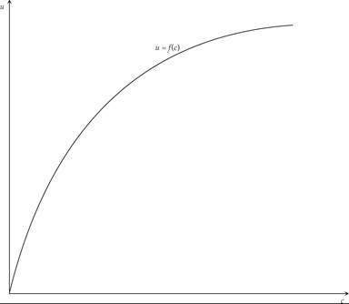
Figure A.1 Utility as a function of consumption.

Consider the case where n is equal to 2. Then a function assigns a unique value y for any vector x = (x₁, x₂)′. An example of such a function is the neoclassical production function of the form

where y denotes the output produced, k the capital stock, and l the labor force. Such a function can be represented graphically as in figure A.2. In the case of a function with n equal to 2, the graph is a surface in three-dimensional space.

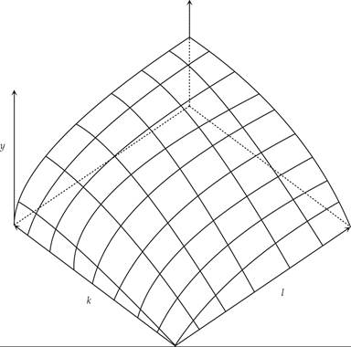
Figure A.2 Output as a function of capital and labor.

As it is not always easy to draw such three-dimensional graphs, we sometimes describe them by holding one of the three variables constant and using a two-dimensional contour map. For example, figure A.3 depicts such a contour map, consisting of isoquants (i.e., combinations of capital and labor that produce a constant volume of output). Higher placed isoquants in the figure correspond to higher output.

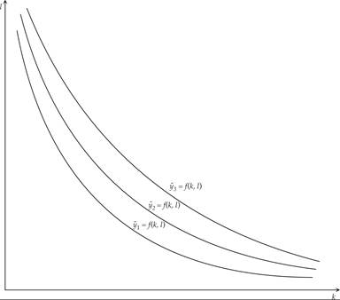
Figure A.3 Isoquants: capital labor combinations that produce given amounts of output.

Figure A.4 depicts another type of contour map, consisting of production functions for given quantities of labor. Each curve depicts the maximum amount of output produced, as a function of the capital stock, for a given quantity of labor. The higher the quantity of labor is, the greater will be the output that is produced as a function of the capital stock. Hence, the higher curves denote relations between output and the capital stock that correspond to higher employment of labor.

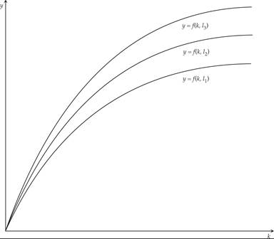
Figure A.4 Output as a function of the capital stock, for a given level of employment of labor.

Functions of vectors of order higher than 2 cannot be represented graphically; they can only be analyzed algebraically.

A.1.2 Derivatives and Partial Derivatives of Functions

The (partial) derivative of a function y = f(x) measures the sensitivity of the function value y to a change in its each of its arguments x. Derivatives are a fundamental tool of calculus.

Consider a function f: ℝ → ℝ. The derivative of the function f(x) evaluated at a point ξ is defined as

The derivative of a function, as a function of x itself, is correspondingly defined and usually denoted as

The f′(x) notation is due to Lagrange, and the notation is due to Leibniz, two of the pioneers of calculus.

Graphically, the derivative is depicted as the slope of a function. It measures the change in the value of the function as a result of an infinitesimally small change in the variable x. Such a change is called a marginal change.

The derivative of the utility function (A.2) is depicted in figure A.5. It measures the effect on consumer utility of an infinitesimally small change in consumption. The derivative of a utility function is called marginal utility. As can be seen from figure A.5, for the utility function depicted, marginal utility is always positive, although declining.

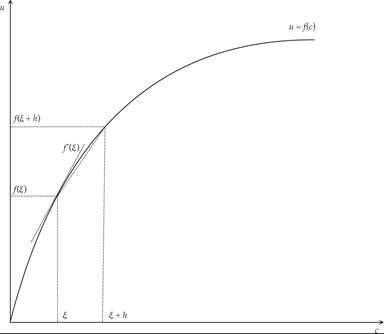
Figure A.5 Utility and marginal utility: the derivative of the utility function.

The process of finding a derivative is called differentiation. The reverse process is called integration. Differentiation and integration constitute the two fundamental operations in calculus.

The derivative of a function can, in principle, be computed from the definition (A.4) by considering the difference quotient and computing its limit. In practice, once the derivatives of a few simple functions are known, the derivatives of other functions are more easily computed using rules for obtaining derivatives of more complicated functions from simpler ones.

Note that if a function is differentiable at a point, it must be continuous at this point. However, even if a function is continuous at a point, it may not be differentiable there. In this text, as in macroeconomics in general, we shall be mostly concerned with continuous and differentiable functions.

The following are the derivatives of some basic functions.

The derivative of a linear function, f(x) = αx, where α is a constant parameter and x is a real variable, is

The proof of this is straightforward:

The proofs for the functions below are based on the same procedure, although they are slightly more involved and will be omitted. However, it is worth knowing the derivatives of the following basic functions.

The derivative of the power function, x^α, where α is a constant parameter and x is a real variable, is

The derivative of the exponential function e^x, where e is the basis of natural logarithms and x is a real variable, is

The derivative of the logarithmic function ln(x) is

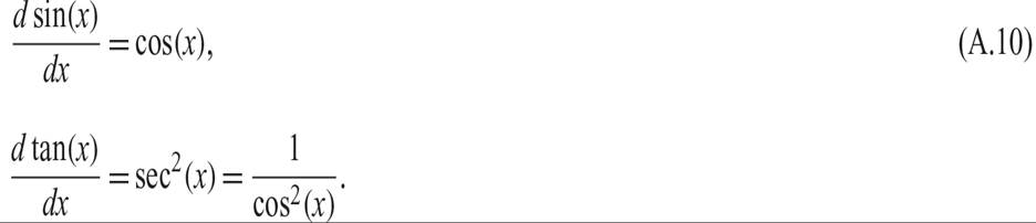
The derivatives of the following trigonometric functions are

The following rules of differentiation can also be proven easily, and they can be applied to sums, products, and ratios of functions, as well as to functions of functions.

The derivative of the sum of two functions f(x) and g(x) is given by the sum of the derivatives:

The derivative of the product of two functions f(x) and g(x) is given by the sum of the products of each function with the derivative of the other:

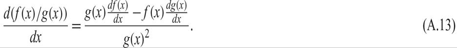
The derivative of the ratio of two functions f(x) and g(x) is given by the difference of the product of the function in the denominator, with the derivative of the other, from the product of the function in the numerator, with the derivative of the other, over the square of the function in the denominator:

Finally, the derivative of a function f of a function g(x), with respect to x, is given by the product of the derivative of f with respect to g, times the derivative of g with respect to x:

Rule (A.14), the rule for differentiating a function of a function, is also called the chain rule.

Partial derivatives of a function with two variables (i.e., f: ℝ² → ℝ) are defined and denoted by

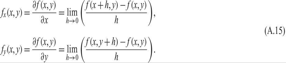
The computation of partial derivatives is straightforward. Simply differentiate with respect to one of the variables, treating the other variable as constant.

The above rule applies equally well to the case of functions with n variables: f: ℝⁿ → ℝ: Partial derivatives are computed by simply differentiating with respect to one of the variables, treating the other variables as constant.

Partial derivatives can be used to totally differentiate a function of n variables with respect to all the variables. Consider the function f: ℝⁿ → ℝ:

The total differential of the function f is determined as

A.1.3 Maxima and Minima of Functions

Consider a function f: ℝ → ℝ. A point ξ at which the derivative of the function is equal to zero is called a stationary point of the function. The reason is that at this point, the function is neither increasing nor decreasing.

Recall from the definition of derivatives that

Hence, if the derivative of a function is equal to zero at a point, the value of the function does not change when x changes.

Figure A.6 shows the stationary points of a general continuous function f(x). The word “stationary” arises from the fact that if one were to place a tiny ball on these points, because the slope is zero and the function is horizontal, the ball would stay in place.

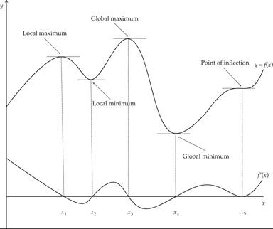
Figure A.6 Stationary points: maxima, minima, and points of inflection.

The figure also shows the graph the derivative function f′(x), which denotes the slope of the original function.

The stationary points of well-behaved function fall into three categories: Local maxima, local minima, and points of inflection. The highest local maximum is called a global maximum, and the lowest local minimum is called a global minimum.

Note that at a local maximum, the slope of the derivative function f′(x) is negative; but at a local minimum, the slope of the derivative function f′(x) is positive. This is equivalent to saying that for a local maximum, the second derivative of the original function f must be negative; for a local minimum, it must be positive. This result is intuitive. For a local maximum, a small change in either direction must result in a reduction in the value of the function. Hence, the derivative function must have a negative slope. For a local minimum, a small change in either direction must result in an increase in the value of the function. Hence, the derivative function must have a positive slope.

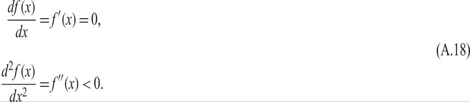
Hence, the conditions for a local maximum of a twice-differentiable continuous function are

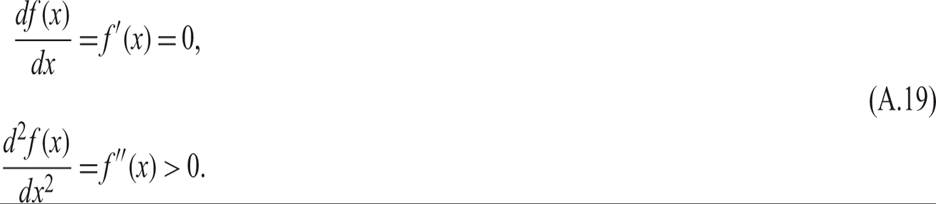
The conditions for a local minimum of a twice-differentiable continuous function are

In most of the applications of calculus in this text, we assume that functions are twice differentiable. Hence, their second derivatives exist and can be computed.

A twice-differentiable function f(x) is concave on an interval if and only if its derivative function f′(x) is monotonically decreasing on that interval; that is, f′′(x) < 0 on that interval. Thus, a concave function has a decreasing slope or first derivative.

A twice-differentiable function f(x) is convex on an interval if and only if its derivative function f′(x) is monotonically increasing on that interval; that is, f′′(x) > 0 on that interval. Thus, a convex function has an increasing slope or first derivative.

These definitions can help us define points of inflection. Points of inflection are points where a function turns from concave to convex, or vice versa. Thus, local maxima are likely to be found in concave functions, or concave intervals of functions, while local minima are likely to be found in convex functions, or convex intervals of functions.

The conditions for the existence of stationary points can be generalized to functions of multiple variables. Consider the following function f: ℝⁿ → ℝ:

A stationary point exists where

Whether the stationary point is a maximum or a minimum depends on the whole array of second partial derivatives of the function. This is a discussion that we shall postpone until we discuss the properties of matrices and linear algebra (appendix B).

A.2 Mathematical Optimization under Constraints

Economics is defined as the study of making the best use of scarce resources. Mathematically, this can be implemented by maximizing some objective function, which measures consumer welfare or the profits of firms, subject to another function, which measures the scarcity of resources.

A.2.1 Constrained Optimization in the Case of a Function of One Variable

Let us first consider the problem of choosing a single variable x to optimize an objective function f(x), under a constraint g(x) ≤ 0. The function to be optimized, called the objective function, is denoted by

Assume that f is a concave function. We shall thus seek to maximize it.

In general, the constraint is a function of the form

The problem then is to find the value of x that maximizes f(x), subject to the constraint g(x) ≤ 0.

Assume that the constraint is satisfied with equality at some value . Then the maximum is attained at if the first derivative of f() is positive. If the first derivative of the function f(x) becomes equal to zero before is reached (say, at point x₀), then the maximum is attained at x₀, before the constraint becomes binding.

Thus, at the optimum, the slope of the objective function f′(x) is equal to the marginal value of the constraint g′(x). With a binding constraint, this value is positive (i.e., the constraint has value); but with a nonbinding constraint, it is equal to zero (i.e., the constraint has no value).

The rule for finding the maximum of a concave function (such as (A.22)), subject to a constraint (such as (A.23)), is to evaluate the first derivative of the function (A.22) at the value of x for which g(x) = 0. If the first derivative is positive, then the constraint is binding and is satisfied with equality. Otherwise, the constraint is nonbinding, and the objective function is maximized before the constraint becomes binding.

Hence, if f′() > 0, the maximum is attained at x = , where is the value of x for which g(x) = 0. If f′() < 0, the maximum is attained at x₀ < , where x₀ is the value of x that satisfies f′(x₀) = 0.

This case is depicted in figure A.7. For a binding constraint, the constrained maximum is obtained to the left of x₀, and the value of the objective function is lower than the value when the constraint is not binding. For a binding constraint, the first derivative of the function f′(x) is positive at the optimum, whereas for a nonbinding constraint, it is equal to zero.

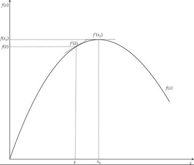
Figure A.7 Maximization with a binding and a nonbinding constraint.

A.2.2 Optimal Consumption under an Income Constraint

A typical economic example is consumer choice under an income constraint. Assume that the consumer maximizes the utility function

subject to the constraint

The constraint can be expressed as

Assume that f′(x) is positive throughout (i.e., that the preferences of the consumer are characterized by nonsatiation) and that marginal utility is always positive. Also assume that f′′(x) < 0 (i.e., that marginal utility is diminishing as the level of consumption increases). Then, by consuming all her income w, the consumer maximizes her utility. The income constraint is binding. The consumer chooses c = w to maximize utility.

The case is depicted in figure A.8. At the maximum, the marginal utility of consumption is equal to f′(w), which is positive throughout. The marginal utility of consumption at the maximum measures the marginal value to the consumer of an extra unit of income. If the income of the consumer were to rise from w₀ to w₁, then the consumer would increase her consumption correspondingly, and the marginal utility of consumption would fall. Thus, the marginal value of income to the consumer would also fall.

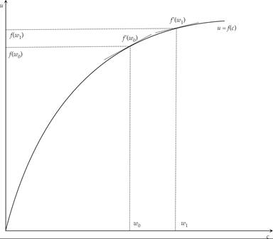
Figure A.8 Maximization of consumer utility subject to an income constraint.

Under the assumption of nonsatiation (i.e., positive marginal utility of consumption at all levels of consumption), the constraint will always be binding, and the household will consume all its income.

A.2.3 The Lagrange Method

The first-order conditions for a maximum of (A.20), subject to constraints such as (A.21), can be derived by a method proposed by Lagrange, which generalizes to all problems of optimization under constraints.

The method consists of constructing a new function, the Lagrange function:

Setting the first derivative of the Lagrange function equal to zero, we get the first-order conditions for an optimum. Here λ is called the Lagrange multiplier, and its interpretation is as the marginal value of the constraint g(x) in terms of the objective function f(x).

Using the chain rule of differentiation, the first derivative of (A.27) is equal to zero when

At the optimum, the first derivative of the objective function with respect to x is equal to the Lagrange multiplier λ times the first derivative of the constraint with respect to x.

Applying the Lagrange method to the consumer problem of maximizing the utility function (A.22) subject to the constraint (A.23), we get that at the optimum.

Thus, at the optimum, the marginal utility of consumption f′(c) is equal to the marginal valuation of income λ. If the marginal utility of consumption is always positive (nonsatiation), then the marginal valuation of income is also positive, and the constraint (A.25) is satisfied with equality. The household consumes all of its income w.

Because we have assumed that f is a concave function, the second derivative of the Lagrange function at the optimum is given by

From (A.30), it follows that the optimum is indeed a maximum. Consumer welfare (A.24) is maximized subject to the income constraint (A.25).

The Lagrange method can be generalized to problems with n variables. Consider the optimization of the objective function

subject to the constraint

Then the first-order conditions for an optimum can be found by optimizing the Lagrange function:

The first-order conditions for an optimum of (A.33) are

for all i = 1, 2, …, n. At the optimum, the first derivative of the objective function with respect to each x_i is equal to the Lagrange multiplier λ times the first derivative of the constraint with respect to each x_i.

We can apply the Lagrange method to a two-variable example from consumer theory. Assume a household who faces exogenous prices of two consumer goods p₁ and p₂, and has an exogenous endowment of money income w. The objective function to be maximized is a utility function given by

where f₁, f₂ > 0, f₁₁, f₂₂ < 0 denote its first and second derivatives with respect to the two consumer goods c₁ and c₂.

Assume that the household maximizes utility subject to

where p₁, p₂ > 0 denote the prices of consumption goods 1 and 2, respectively, and w > 0 denotes the money income of the household.

We seek the first-order conditions for the maximization of (A.35) subject to the income constraint (A.36). The Lagrange function for this problem is given by

From the first-order conditions for a maximum, we have

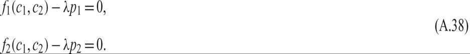
The first-order conditions (A.38) can be rewritten as

id=eqA-39.png class="lazyload" data-src="/files/uch_group77/uch_pgroup317/uch_uch7367/image/image1584.jpg" alt=eqA-39.png>

The economic interpretation of (A.39) is straightforward. At the maximum, the marginal utility of each of the two goods is equal to the marginal value of money income λ (the Lagrange multiplier) times the price of each good in terms of money.

Because marginal utilities and prices are assumed positive, the marginal value of money income λ will also be positive. Thus, the constraint will be binding and will be satisfied with equality. The household will spend all of its money income, and we have that

The three unknowns, c₁, c₂, and λ, can be found by solving the system of the three equations (A.39) and (A.40). Thus, optimal consumption and the optimal marginal value of money can be found as functions of the exogenous set of prices p₁ and p₂ and money income w.

The optimality conditions can be given another interpretation, known from intermediate microeconomics. Dividing the first by the second equation in (A.39), we eliminate λ between the two equations, resulting in

The economic interpretation of (A.41) is that at the optimum, the ratio of the marginal utilities of goods 1 and 2 is equal to their relative price. The ratio of the marginal utilities is equal to the marginal rate of substitution between the consumption of goods 2 and 1. Hence, at the optimum, the marginal rate of substitution between the two goods is equal to their relative price.

To further delve into this interpretation, we can totally differentiate both the objective function (A.35) and the budget constraint (A.40).

Totally differentiating the objective function (A.35) results in

For a constant level of utility, df = 0. The marginal rate of substitution between the consumption of good 2 and the consumption of good 1 is thus given by

The marginal rate of substitution, (i.e., the marginal change in the consumption of good 2 required to maintain a constant level of utility following an infinitesimally small change in the consumption of good 1) measures the slope of indifference curves. It is negative and equal in absolute value to the ratio of marginal utilities of good 1 and good 2.

By totally differentiating the budget constraint (A.40), we get that

For a constant level of income, dw = 0. Therefore, it follows from (A.44) that

Equation (A.45) measures the slope of the budget constraint (A.40). It denotes how much of good 2 the household has to sacrifice to buy an extra unit of good 1.

Thus, the optimum is determined at the point where the budget constraint touches the highest possible indifference curve. At this tangency point, the slope of the budget constraint and the indifference curve of the household coincide.

The determination of the optimum is depicted in figure A.9. At the optimum (i.e., point E, the consumption bundle that maximizes the utility of the household), the marginal rate of substitution (i.e., the slope of the highest possible indifference curve) is the same as the relative price of the two goods, which is the slope of the budget constraint.

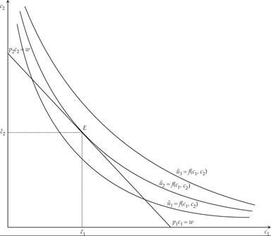
Figure A.9 Optimal choice of a consumption bundle.

A.3 Some Useful Functional Forms

This section introduces some useful functional forms and discusses their properties. These functional forms are widely used to model either the production process or the preferences of households. We shall focus on the constant elasticity of substitution (CES) production and utility functions and the constant elasticity of intertemporal substitution (CEIS) utility function.

The CES functional form contains other functional forms as special cases, such as the Cobb-Douglas, fixed proportions, and linear production and utility functions.

The CEIS functional form is a relatively general additive functional form, which is quite useful in modeling intertemporal preferences and uncertainty. It contains the logarithmic, linear, and quadratic utility functions as special cases.

A.3.1 The Two-Factor CES Production Function and the Elasticity of Substitution

The CES production function was introduced by Arrow et al. [1961]. As its name suggests, it is a production function for which the elasticity of substitution between capital and labor is constant. In its most general form, it can be written as

where A > 0 is total factor productivity, which is assumed to be exogenous and constant. It is assumed that 0 < a, b < 1 and ψ < 1 are constant parameters. Their interpretation will become apparent shortly.

By multiplying both inputs by any positive λ, it is straightforward to confirm that this production function exhibits constant returns to scale.

The technical rate of substitution measures how one of the inputs (say, labor) must adjust to keep output constant, when the other input (say, capital) changes. In the two-factor case, it is just the slope of the isoquant and is defined by

where F_K and F_L are respectively the marginal products of capital and labor at output Y.

The elasticity of substitution σ between capital and labor is defined as the percentage change in the ratio of labor to capital, divided by the percentage change in the technical rate of substitution, with output being held fixed. It is a measure of the curvature of the isoquants of the production function. The elasticity of substitution σ is thus defined by

For the CES production function, the technical rate of substitution is given by

Thus, the elasticity of substitution σ is given by

From (A.50), one can confirm that the elasticity of substitution is indeed constant.

A.3.2 Special Cases of the CES Production Function

As ψ tends to minus infinity, the elasticity of substitution tends to zero. Thus, the CES production function contains as a special case the fixed-proportions production function, with a zero elasticity of substitution between capital and labor. This takes the form

Equation (A.51) is a production function that was widely used prior to the introduction of neoclassical production function, by, for example, Harrod [1939], Leontieff [1941], and Domar [1946]. It is often referred to as the Leontieff production function.

As ψ tends to zero, the elasticity of substitution tends to one. It is straightforward to show, using L’Hopital’s rule, that in this case, the limit of the CES production function is the Cobb-Douglas production function. This functional form, due to Cobb and Douglas [1928], is used extensively in macroeconomics. It is worth remembering that it is a special case of the CES production function, with a unitary elasticity of substitution between capital and labor. It takes the form

where A = Ab^a(1 − b)^1−a

Finally, for ψ = 1, the CES production function becomes linear, and the elasticity of substitution between capital and labor becomes infinite. Thus, the CES production function contains the linear production function as a special case.

A.3.3 The CES Production Function and the Solow Model of Economic Growth

Expressing the CES production function per efficiency unit of labor, one gets

The marginal product of capital (per efficiency unit of labor) is then given by

The average product of capital (per efficiency unit of labor) is given by

One can confirm from (A.54) and (A.55) that for any ψ < 1, both the marginal and average products of capital (per efficiency unit of labor) fall as capital per efficiency unit of labor increases. Thus, the CES production function is characterized by diminishing returns to capital accumulation. The question that arises is whether the Inada conditions are satisfied in the case of the CES production function.

Consider first the case 0 < ψ < 1, that is, an elasticity of substitution between capital and labor that is greater than one. The limits of the marginal and average products of capital, as capital tends to zero and infinity, respectively, are given by

Thus, in the case of an elasticity of substitution that is greater than one, the CES production function does not satisfy the second Inada condition, and a steady state capital stock (per efficiency unit of labor) may not exist.

For example, in the Solow model, if

then steady state does not exist, and capital per efficiency unit of labor grows continuously. The model becomes one of endogenous growth.

Consider next the case ψ < 0, that is, an elasticity of substitution between capital and labor which is lower than one. The limits of the marginal and average products of capital, as capital tends to zero and infinity, respectively, are given by

Thus, in the case of an elasticity of substitution that is less than one, the CES production function does not necessarily satisfy the second Inada condition, and a steady state capital stock (per efficiency unit of labor) may not exist.

For example, in the Solow model, if

then a steady state does not exist, and capital per efficiency unit of labor is driven to zero.

Only in the case where the constant elasticity of substitution between capital and labor is equal to one (that is, the Cobb-Douglas case) is the satisfaction of both Inada conditions—and hence the existence of a steady state—guaranteed.

A.3.4 The CES Utility Function

The CES functional form can also be used for modeling consumer utility. Assuming a household that has access to two goods, c₁ and c₂, the CES utility function takes the form

where α is the relative weight of good 1 in the utility of the consumer. Equation (A.56) has the same properties as the two-factor CES production function (A.46).

The elasticity of substitution in the consumption of the two goods is constant and given by 1/(1 − ψ). As ψ tends to minus infinity, the elasticity of substitution tends to zero. Thus, the CES utility function contains as a special case the fixed-proportions utility function, with a zero elasticity of substitution between the two goods. As ψ tends to zero, the elasticity of substitution tends to one. It is straightforward to show, using L’Hopital’s rule, that in this case, the limit of the CES utility function is the Cobb-Douglas utility function. Thus, the CES utility function contains the Cobb-Douglas utility function as a special case, with a unitary elasticity of substitution between the two goods. Finally, for ψ = 1, the CES utility function becomes linear, and the elasticity of substitution between the two goods becomes infinite. Thus, the CES utility function contains the linear utility function as a special case.

The CES functional form can be generalized to n goods. Assuming a household that has access to n goods, a CES utility function in which good i has a weight in consumer utility equal to α_i > 0, takes the form

The elasticity of substitution in the consumption of any two goods among the n goods is constant and given by 1/(1 − ψ).

A.3.5 Additively Separable Utility and the CEIS Utility Function

Because utility functions are defined up to any monotonic transformation, we can raise the CES utility function (A.57) to the power ψ. We then end up with a utility function of the form

The difference between the CES utility function (A.57) and the CES utility function (A.58) is that (A.58) is an additively separable utility function. Unlike the original CES utility function (A.57), the marginal utility of consumption of each good in (A.58) is independent of the consumption of the other goods. This property is defined as additive separability.

Taking the first derivative of the original CES utility function (A.57) with respect to c_i, the marginal utility of good i is given by

Taking the first derivative of the transformed CES utility function (A.58) with respect to c_i, the marginal utility of good i is given by

In the case of the original CES utility function, the marginal utility of consumption of good i depends on the consumption of all other goods. But in the case of the transformed CES utility function, it only depends on the consumption of the good itself.

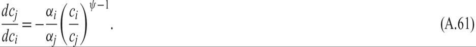
However, this does not affect consumer choice. For both the original and the transformed CES functions, the marginal rate of substitution between the consumption of any two goods i and j, and hence the slope of indifference curves, is given by

It is in this sense that utility functions are defined up to a monotonic transformation.

The differences between (A.57) and (A.58) do not matter for the optimal choice of the consumption bundle. Given that at the maximum, the marginal rate of substitution is equal to the relative price of the two goods, consumer choice is the same for both the original and the transformed CES utility functions. For any two goods i and j, it is determined by

Additively separable utility functions are used extensively in intertemporal macroeconomics. The presumption is that the marginal utility of consumption in one period does not depend on the level of consumption in previous or future periods.

Thus, a monotonic transformation of a version of the CES utility function (A.57), in which (A.57) is raised to the power ψ, and multiplied by 1/ψ, is a widely used functional form for intertemporal utility functions. It takes the form

where c_t denotes consumption in different time periods, t = 0, 1, …, T; and ρ > 0 denotes the rate at which the household discounts the future, which is called the pure rate of time preference. Thus, relative to (A.58), in (A.63), α_t = (1/(1 + ρ)^t. In the equation, θ = 1 − ψ is the inverse of the elasticity of substitution, 1/θ is the elasticity of intertemporal substitution in this context, and the utility function of the form of (A.63) is termed the constant elasticity of intertemporal substitution (CEIS) utility function.

It is straightforward to show that if θ, and the elasticity of intertemporal substitution 1/θ, are equal to unity, then (A.63) is not defined. Because U is not defined when θ is equal to unity, we might as well consider what happens to the first derivative of U with respect to c_t as θ tends to unity. This is the essence of L’Hopital’s rule. If the first derivative is defined and is the first derivative of a known function, then the original functions tends to that particular function as θ tends to unity. In this case, we have that the limit of the first derivative of (A.63) is given by

where 1/c is the first derivative of a logarithmic function. Hence, L’Hopital’s rule implies that as θ tends to unity, the CEIS utility function tends to the intertemporal logarithmic utility function:

This is often used in intertemporal macroeconomics as a special case of the CEIS utility function.

Two extreme cases of (A.63) are worth mentioning, although they are not widely used. The first is the limit of (A.63) as θ tends to 0 and the elasticity of intertemporal substitution tends to infinity. Then the CEIS utility function becomes a linear intertemporal utility function of the form

The second is the limit of (A.63) as θ tends to infinity and the elasticity of intertemporal substitution tends to zero. Then the CEIS utility function becomes independent of consumption.

1. For rigorous introductions to calculus for economists, see Binmore [1983], or another comprehensive textbook of mathematics for economists, such as Chiang [1974], Simon and Blume [1994], or Klein [2013]. For full discussions of optimization under constraints suitable for economics, see Intriligator [1971] and Dixit [1990].