MODELING THE SOURCES OF MACRO INEQUALITY

In this section we show what macroeconomics has to say about inequality. We start by exploring in Section 14.2.1 the implications of existing macro models for the distribution of wealth.

14.2.1 Theories of Wealth Inequality Given the Process for Earnings

We start this section by emphasizing the limits of the neoclassical growth model with infinitely lived agents and complete markets in predicting wealth inequality. After reviewing the prediction of the overlapping generations model, we analyze models with incomplete markets. As we will see, the consideration of market incompleteness allows for more precise predictions about the distribution of wealth for given processes of indi­vidual earnings.

14.2.1.1 The Irrelevance of Income and Wealth Inequality in the Neoclassical Model The deterministic neoclassical growth model says very little about income and wealth inequality. Note that we mean the neoclassical growth model in its modern meaning of incorporating fully optimizing saving behavior.^[13] In an important article by Chatterjee (1994), reiterated later by Caselli and Ventura (2000), it is shown that any ini­tial distribution of wealth is essentially self-perpetuating. To see this, consider the typical problem of a household i 2 {1,..., I}. Using recursive notation with primes denoting next period variables, the household’s problem can be written as

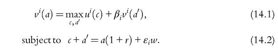
Here, u’(c) is a standard utility function (differentiable, strictly concave), β_i 2 [0,1] is the discount factor, and ε_i is the household’s endowment of efficient units of labor, which we assume constant for now.

where u^t_c(c,) is the marginal utility of consumption. In steady state, the allocation is con­stant over time, c_i = c_i∙', and r = r', which requires that the rate of return on savings is equal to the rate of time preference in every period, that is, β_i = (1 + /)1. One implication is that, if households have interior first order conditions so that Equation (14.3) is satisfied with equality, then β_i = β for all i. Otherwise, some households would reduce their assets as much as they can until they reach some lower bound that depends on the borrowing ability.

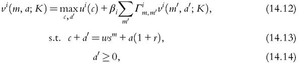
Because the rate of return in the neoclassical growth model is given by the marginal productivity of capital, we have that

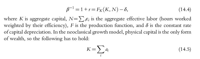
where a_i are the assets held by household i. Note that these last three equations are the only ones imposed by the theory. It turns out that any distribution of wealth {α_i}¹=₁ that satisfies Equations (14.4) and (14.5) is a steady state of this economy in which each indi­vidual household i consumes its income, c_i = ar + ε_iw. This is the sense in which the theory poses no constraints whatsoever on the distribution of α. Note that this is true no matter how efficiency units of labor (and hence earnings) are distributed across households. Nonseparability between consumption and leisure does not change this finding.

Small details qualify the behavior of the system outside a steady state. Under constant relativerisk-aversion (CRRA) preferences, Equation (14.3) can be written as 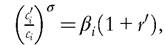whereis the intertemporal elasticity of substitution.

What other possibilities does the neoclassical growth model or its variants offer? Not many. Consider heterogeneity in the per period utility function. We have already noted that this does not change any steady-state consideration. Outside the steady state, the model just takes the initial wealth distribution and uses the first order conditions and the budget constraints to propagate the wealth distribution into the future, essentially dis­persing or concentrating the wealth distribution without much endogenous action on the part of the model.

What about stochastic versions of these economies? With complete markets, all idi­osyncratic uncertainty disappears (it is insured away), whereas the aggregate uncertainty is borne by those who are more willing to bear it. If such ability to bear the risk is increasing in wealth, then the model could generate some redistribution in response to aggregate shocks. But abstracting from aggregate uncertainty, we will see that the irrelevance result no longer applies when markets are incomplete (and agents continue to face idiosyncratic shocks). Before exploring the implications of incomplete markets, however, we briefly review the overlapping generations model.

14.2.1.2 Overlapping Generations Models and Wealth Inequality

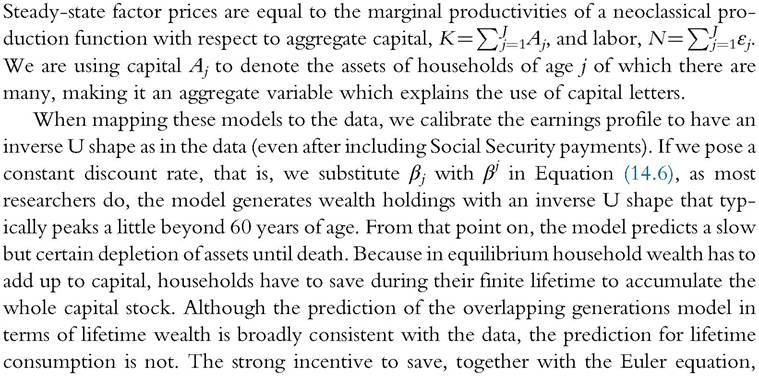
In overlapping generations models, new households are born every period and live up to a certain number of periods J (they may also die earlier with some probability).⁴ In what follows, we abstract from differences among households in any given age cohort and assume that the heterogeneity is only between cohorts. House­holds in age cohort j have earnings ε_j∙, which we take as exogenous. This specification can accommodate retirement and, with some extra work, government-provided Social Security (see Section 14.2.2 for theories of the determination of age-specific earnings).

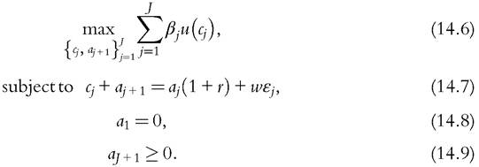
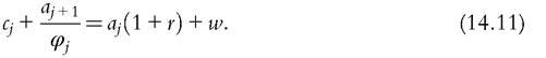
Here, βj is the specific weight that households place in the age-j utility. Note that house­holds are born with no assets and cannot die with debts. Steady-state factor prices are r and w. The solution of the problem includes age-specific consumptions, c,∙, and asset holdings, O_j, that satisfy the Euler equation

^[1] Sometimes the literature uses the term “overlapping generations model” for environments in which new agents are born every period and die with some probability at any point in the future. We refer to this particular environment as the Blanchard-Yaari model (Blanchard, 1985; Yaari, 1965), which is very similar mathematically to the infinitely lived model.

implies that c_j+1 > Cj for all j. In the data, however, consumption is also hump shaped. Var­ious approaches are proposed in the literature to get around this shortcoming. They include demographic shifters, nonseparable leisure in the utility function (Auerbach and Kotlikoff, 1987; Rios-Rull, 1996), existence of both durable goods and incomplete financial markets (Fernandez-Villaverde and Krueger, 2011), borrowing constraints and low rates of return (Gourinchas and Parker, 2002), and others.

With stochastic mortality, the model produces identical predictions as long as there is a market for annuities (which are available even if scarcely used). To see why, consider the probability of surviving between ages j and j + 1, which we denote by φj. The survival probability multiplies the discount factorcapturing the fact that the household gets utility only if alive.^[14] Fairly priced (i.e., issued at zero expected cost) annuities imply that households save by purchasing them, and one unit of savings today yields (1 + r) units of the good tomorrow if the household survives and zero otherwise.

It can be verified that with these modifications to discounting and the budget constraint, we obtain the same first order conditions as in Equation (14.10).

Ifwe assume that there are no annuities, as in Hansen and Imrohoroglu (2008), we have to make some assumption about the allocation of the assets left by the deceased households. There are various options. One possibility is to assume that any household is like a pharaoh and assets are buried with their owners. The predictions of the model change a little relative to the basic model because there is now a smaller amount of total wealth due to the lower rate of return tilting the allocation toward young ages. Other options include the assumption that there is a 100% estate tax (with implications identical to that of the pharaoh model except for the use of public revenues) or that the assets of the deceased go to those in a certain age group. If the assets are distributed equally among the households of certain age groups, the wealth distribution will present a hike at the age at which households inherit, which is not a feature ofthe data. A more attractive alternative that has not been directly explored is to build direct links between a dead household and a randomly chosen younger household that inherits the assets. In this case, there will be limited within-cohort inequality that results from differences in the timing of the death and the wealth of the ancestors.

What about versions of overlapping generations economies with aggregate shocks? With aggregate shocks, even if there are markets for one-period-ahead state-contingent assets, there could be incomplete insurance because households that are not alive cannot insure each other. The answers depend first on the size of the shocks. For (small) business­cycle type shocks, there are no great differences between the allocations implied by complete or incomplete markets.

If markets for the insurance of idiosyncratic risks are not present and households can save only by holding noncontingent assets, the situation changes dramatically and the model has very tight predictions. We will see this in the next section.

14.2.1.3 Stationary Theories of Earnings and Wealth Inequality

When households do not have access to insurance against shocks, the accumulation of riskless assets acts as a mechanism that allows households to smooth consumption—saving in good times when earnings are above the mean and dissaving in bad times. This means that in environments in which households are subject to uninsurable risks, those that have been lucky and have enjoyed good realizations of the shocks are wealthier than those that faced adverse realizations. This type of ex post inequality has been widely studied in models in which the risk was on endowments or earnings and agents could save only in the form of non-state-contingent assets. The basic theory was first developed in Bewley (1977), and the general equilibrium and quantitative properties were studied later by Imrohoroglu (1989), Huggett (1993), and Aiyagari (1994). These ideas have impor­tant applications such as those in Carroll (1997) and Gourinchas and Parker (2002).

Successive studies have extended these models to improve the ability to generate greater wealth inequality. Among these approaches are the addition of special earning risks (Castafieda et al., 2003), entrepreneurial risks (Angeletos, 2007; Buera, 2009; Cagetti and De Nardi, 2006; Quadrini, 2000), endogenous accumulation of human cap­ital (Terajima, 2006), and stochastic discounting (Krusell and Smith, 1998). Because in these models inequality is endogenous, the degree of wealth concentration can be affected by policies. This opened the way to studies that investigate the importance of taxation policies for wealth inequality. Examples are Dlaz-Gimenez and Pijoan-Mas (2011), Cagetti and De Nardi (2009), and Benhabib et al. (2011).

We start by reviewing how to pose the process for earnings (Section 14.2.1.3.1), and then we describe the main features of the Aiyagari model (Section 14.2.1.3.2).

14.2.1.3.1 Stochastic Representation of Earnings

A large body of literature tries to provide a parsimonious representation of the stochastic processes for wages or earnings. This literature uses panel data to estimate a univariate process for labor income or earnings, sometimes at the level of individual earners and sometimes at the household level (which is more in line with the data used in Tables 14.1 and 14.2).^[15] (See, for example, Guvenen, 2009 or Guvenen and Kuruscu, 2010; Guvenen and Kuruscu, 2012.)

One important feature to take into account, as we will see below, is that the most common data sets do not include the very rich. The SCF is designed to provide a better picture of the rich but, unfortunately, it has no panel dimension and therefore cannot be used to separate individual effects from shocks and other interesting property that affects the most appropriate representation of earnings as a stochastic process. A comparison between the properties of the cross section in both data sets gives an idea of the differences in the sample. Recent work using either tax data (Atkinson et al., 2011; DeBacker et al., 2011) or Social Security data (Guvenen et al., 2012) looks very promising in terms of including both the very top earners and information about the persistence of their earnings.

14.2.1.3.2 The Aiyagari (1994) Model

Households do not care for leisure and assess consumption streams through a per period utility function u^t(c) with intertemporal discount factor β_i. The utility function and the discounting may be type specific.

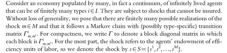
We start by considering the most primitive financial structure in which households have access to saving only in one-period noncontingent assets, and they cannot borrow. To map the model to a real economy and to consider its empirical implications, we build the model economy on top of a neoclassical growth model with exogenous labor supply. With a Cobb-Douglas production function, the prices of capital (rental rate of capital) and labor (wage) depend only on the capital-labor ratio. Because the aggregate labor sup­ply is constant, prices depend only on aggregate capital K, and we can express them as r(K) and w(K).

We consider only steady-state equilibria in which households face a constant interest rate r and a constant wage w per efficiency unit of labor. This approach is common in these types of studies because it greatly simplifies the computational burden. In fact, by focusing on steady states, when we solve the individual problem we can ignore the evolution of the aggregate states and we only need to keep track of the individual states (household’s type i, asset position a, and realization of the idiosyncratic shock m). Of course, by doing so we have to exclude from the analysis changes that affect the whole economy, such as aggregate productivity shocks or structural changes. The consideration of aggregate and recurrent shocks represents a major computational complication (see, for example, Krusell and Smith, 1998). However, if we restrict ourselves to explore the implications of a one-time completely unexpected shock (a somewhat oxymoronic term) or structural change, then the computation remains tractable. For simplicity of exposi­tion, we limit the analysis here to steady-state comparisons with the caveat that in the real economy, the distribution will take a long time to converge to a new steady state.

The household’s problem can be written as

where the superscript i denotes the household’s type. Because this does not vary over time, we wrote it outside the arguments of the value function. The first order condition is given by

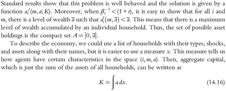
The measure x gives us all the information that we need. For example, the total amount of efficiency units of labor or aggregate labor input is equal to

To calculate the Gini index for wealth, we need to compute the Lorenz curve and then calculate its integral. Note that any point of the Lorenez curve, for example, its value at 0.99 denoted by ‘₀₉₉, is one minus the share of wealth held by the richest 1%. To com­pute ‘0.99, we start by finding the threshold of wealth that separates the richest 1% from the rest of households. Once we have found the threshold, we compute the wealth held by those households with wealth above the threshold relative to total wealth. The Gini index is simply twice the area between the Lorenz curve and the triangle below the diag­onal between 0 and 1. (See Figure 14.6, for instance.) Other inequality statistics are also readily obtained from x, including those pertaining to the joint distribution of earnings and wealth and their intertemporal persistence.

The Aiyagari model has unique predictions about wealth and income inequality for any specification of the process of earnings. Therefore, the determination of the prop­erties of the earning process becomes the central issue in the application of this model to the data. Should we think of people as being all ex ante equal in the sense that there is only one i type and they differ only in the realization of the shock? Or should we think of people consisting of different ex ante types? In either case, how do we determine which process to use? We now turn to this issue.

As we have seen in Section 14.1, the distribution of wealth in the United States is highly skewed, with about one-third of all the wealth in the hands of a mere 1% of house­holds. How did those households become so wealthy? In order to become rich, house­holds need both motive and opportunity. The reason for the opportunity is clear: at some point, the households had to have high enough earnings to be able to save and accumulate high levels of wealth. Motive is also important: why should households save rather than consume if they are impatient? Ifhigh earnings are not going to be around forever, then prudent households would want to save for the bad times that are likely to lie ahead. The issue is whether motives and opportunities are big enough to generate the wealth con­centration observed in the United States.

To choose the actual parameterization of the earnings process for the model, we first need a Markovian process for earnings. If the focus is on the U.S. economy, one possi­bility is to specify a process estimated using the Panel Study of Income Dynamics (PSID). This is what Aiyagari (1994) did in his seminal paper, which relied on existing empirical studies such as Abowd and Card (1987) and Heaton and Lucas (1996).

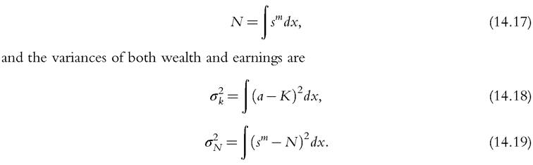
The results are disappointing. The first row of Table 14.6 shows the shares of wealth of key groups in the U.S. data, and the second row displays those same shares as predicted by a model in which the earning process is calibrated using PSID data. The red line in Figure 14.4 shows the associated Lorenz curve. There is very little inequality compared with the inequality observed in the U.S. economy. The shares of wealth of the top 1% and the top quintile generated by the model are 4% and 27%, respectively, whereas in the United States these shares are 34% and 87%. The use of alternative estimates of the earn­ing process, such as those provided by Storesletten et al. (2001), improves the perfor­mance of the model but only marginally.

The model fails to replicate the high concentration of wealth observed in the data for many possible reasons. One obvious explanation is that the model misses important pieces; for example, the model ignores life-cycle heterogeneity with all the demographic complications of actual lives. Or it ignores the permanent characteristics of people as well as education and human capital acquisition. It also ignores the fact that lives are affected by many other types of shocks such as health or unforeseen expenditures.

Castaheda et al. (2003) take a different approach and argue that the reason for the fail­ure is the misrepresentation of the process of earnings. The PSID sample does not include very rich households. A comparison of its data with that of the SCF in which the emphasis is on wealthy people shows a large mismatch. The PSID does a better job at including people outside the top 10% of income earners and asset holders, but it is not appropriate to capture the dynamic properties of the incomes earned by the top of the distribution. Based on this observation, Castaiieda et al. (2003) propose to ignore the PSID and focus instead on the specification of a process for earnings where the cross-sectional dispersion is similar to the SCF but its persistence is engineered so that it replicates the main features of the wealth inequality.

The third row of Table 14.6 displays the wealth distribution of an economy where the earning process has been calibrated following the above criteria. As we can see from the table, the model replicates quite well (by construction) the empirical data. Comparing the two processes for earnings (at least in the parsimonious representation used in Diaz et al., 2003) is very useful. The version of their economy designed to replicate the prop­erties of the original Aiyagari economy has three values for earnings that are essentially symmetric, as are the persistence properties of the process: the earnings of agents in the middle and top thirds are 1.28 ? and 1.63 ?, respectively, the earnings of those of the bottom third. Households in both, the top and the bottom thirds, have a one-third prob­ability of moving out of their current situation by the next period. This society is very equal. Moreover, encountering bad luck, that is, being sent to the bottom third, is not really that bad. Clearly, because there are few motives to save money in this society, households soon stop doing so and consume all of their income.

The process that replicates the U.S. wealth distribution is extremely different from the process just described. The bottom of the society is now almost half of all households. Moreover, once at the bottom, less than 1% of these households move up each year.

Table 14.6 Concentration of wealth of various economies

Aiyagari (1994) usedthe PSID Ear-Pers calibration, Castafieda et al. (2003) used the SCF Ear-Wea calibration, and Krusell and Smith (1998) used both the Emp-Unemp and the Stochastic β calibrations.

U.S. data source Kuhn (2014).

Households that make up the middle class, almost one-half of the population, earn 5 ? more than those at the bottom and have an equal chance (1%) of moving up or down. Only 6% of the households are in the top earnings group, and their earnings are huge: 47 ? those of the poor and 9 ? those of the middle class. More than 8% of these house­holds will move down in a given year. Although these particular values are somewhat arbitrary, they give an accurate sense of how extreme both motives and opportunities have to be in order to induce the U.S. wealth disparities in a model in which agents differ only in the realization of a common earnings process.

Krusell and Smith (1998) pursue a very different approach to get a suitable wealth distribution. Instead of tracking the behavior of earnings, they pose a simple employ- ment/unemployment process to generate earnings inequality, and they assume that the discount rate of individual agents is also stochastic. Therefore, in addition to the idi­osyncratic shock to earnings, they consider a second idiosyncratic shock to the discount rate. The earnings process alone generates almost no inequality because the only way to get rich is through remaining employed but without earning more than other employed workers. In the extension with stochastic discounting, they assume that β can take three values, {0.9858,0.9894,0.9930}, with a symmetric distribution that satisfies the follow­ing properties: (i) the average duration of the extremes is 50 years (so it lasts the length of the adult life of a person); (ii) the transition from extreme to extreme requires a spell in the middle; and (iii) the (stationary) size of the middle group is 80%. Interestingly, the model with stochastic discounting yields disarmingly similar inequality indexes as in the data (see the last row of Table 14.6).

Various papers used life-cycle models with idiosyncratic risk to study wealth inequal­ity. An important early contribution is Huggett (1996). De Nardi (2004), Cagetti and De Nardi (2006), and Cagetti and De Nardi (2009) study the role of bequest, estate tax­ation, and entrepreneurship in shaping the wealth distribution.

14.2.2 Theories of Earnings Inequality

So far we have described how macroeconomists think of the distribution of wealth given the distribution of earnings. But what about the distribution of earnings itself? Where is it coming from? In general, we can think of the differences in earnings as resulting from a combination of heterogeneity in (i) innate abilities or ex ante luck that persists for the lifetime of the agent; (ii) ex post luck due to the realization of shocks that are not under the control of the agent; (iii) effort or occupational choice; and (iv) investment in human capital. In the model considered in the previous section, the heterogeneity in earnings was only a consequence of innate heterogeneity (captured by the agents’ type) and ex post luck (captured by the Markov process for skills). In this section we make the earnings endogenous by allowing for the optimal choice of effort and investment in human capital. An important consequence of endogenizing the earning process is that the distribution of earnings can be affected by several factors including financial market development (which, for example, facilitates access to the financing of investment in human capital) and taxation policies (which, for example, affect the marginal decision of effort and investment in human capital).

Next we briefly describe three aspects of models with endogenous earnings: models in which earnings are the result of explicit choices of either learning by doing or learning by not doing, including education (Section 14.2.2.1); models in which not all types oflabor are perfect substitutes (Section 14.2.2.3); and models with occupational choices in which agents decide which occupation to take (Section 14.2.2.5).

14.2.2.1 Human Capital Investments

A common approach to endogenizing the process for earnings is the assumption that human capital is endogenous and depends on the individual investment chosen by agents. If the return from the investment is stochastic, then agents will be characterized ex post by different levels of human capital and, therefore, unequal earnings. An interesting feature of this setup is that it generates a positive relation between the aggregate performance of the economy and the degree of inequality. More specifically, higher investment in human capital leads to higher income or growth or both, but also to higher inequality because investment amplifies the impact of idiosyncratic shocks.

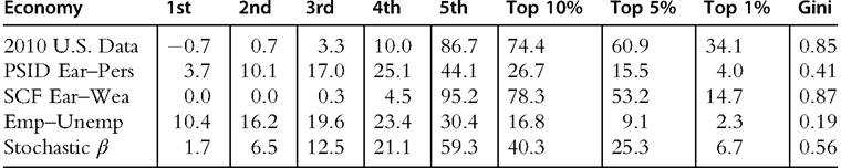
We illustrate this point with a simple model without taking a stand on the issue of what type of investment yields higher human capital. The investment can be either the result of time and hence forgone output or leisure, or the result of effort that generates a disutility, or the result of investment in goods. In this sense and at this level of abstrac­tion, it accommodates both learning by direct investment in schooling or more general human capital investment such as that pioneered by Ben-Porath (1967). It also captures the key mechanisms formalized in more recent studies such as Guvenen et al. (2009), Manuelli and Seshadri (2010), and Huggett et al. (2011). For an extensive discussion of the life-cycle human capital model, see von Weizsacker (1993).

Consider an economy with a continuum of risk-neutral workers, each characterized by human capital h. Production, which in this simple model corresponds to earnings, is equal to the worker’s human capital h. Individual human capital can be enhanced with investment captured by the variable y. Investment is costly in terms of either utility or

Because the outcome of the investment is stochastic, the model generates a complex distribution of human capital among workers. In the long run, the distribution will be degenerate because at the individual level h follows a random walk. To make the distri­bution stationary and keep the model simple, we assume that workers die with proba­bility λ in each period and are replaced by the same mass of newborn workers. To allow for ex ante heterogeneity or innate abilities, we also assume that newborn agents are heterogeneous in initial human capital. In particular, there are I types of newborn agents indexed by i 2 {1,..., I}, each of size x0 and with initial human capital h^t₀. The initial distribution of newborn agents satisfies

Because of the linearity assumption, it will be convenient to normalize by h the opti­mization problem solved by a worker. We can then write the problem recursively as 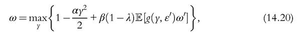where ω is the expected lifetime utility normalized by human capital h. The non­normalized lifetime utility is ωh. Of course, the linearity of the accumulation function is crucial here. Ifthe new human capital was a Cobb-Douglas function of old human cap­ital, as in the Ben-Porath (1967) model, the analysis would be more complex analytically.

The first order condition gives

whereis the average value of the stochastic variable ε.

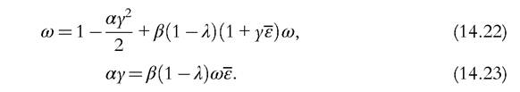
Because the first order condition is independent of h, the investment variable y is con­stant over time, which in turn implies that the normalized lifetime utility for the worker, ω, is constant. Therefore, y and ω can be determined by the two equations that define the value for the worker and the optimal investment, that is,

Given the distribution of human capital for newborn workers xo and the investment var­iable y, we can determine the economy wide distribution of human capital (equal to the distribution of earnings) and compute a cross-sectional index of inequality. We focus on the square of the coefficient of variation, that is,

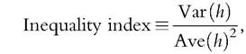
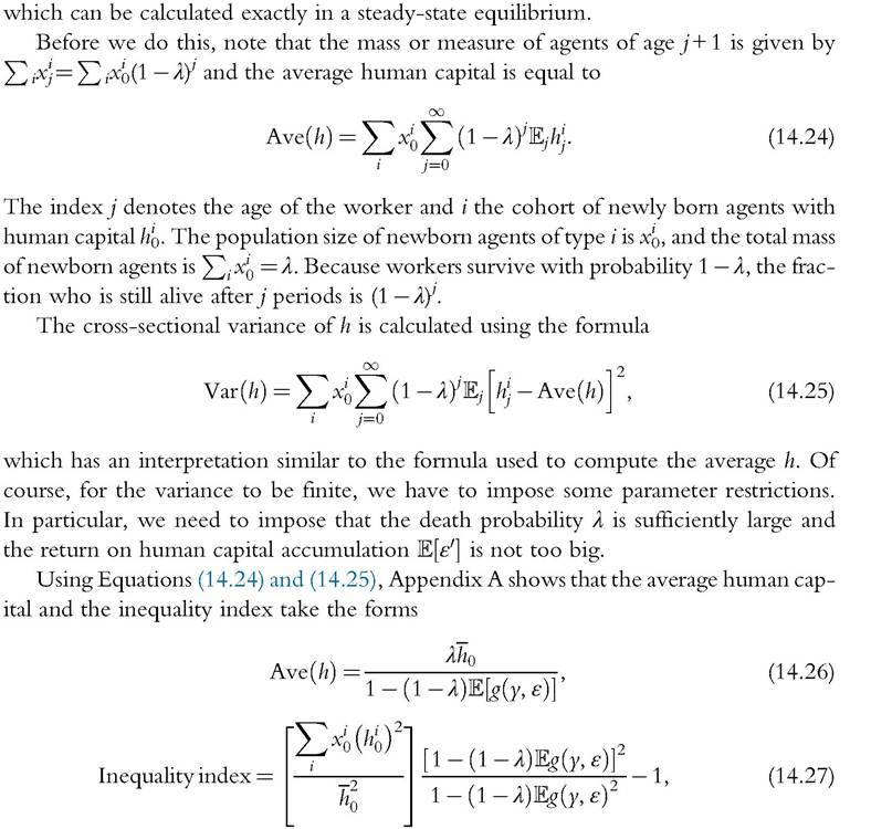
where h₀ is the aggregate human capital of newborn agents.

We can see from Equation (14.26) that the average human capital and, therefore, aggregate output are strictly increasing in the investment variable y. This is intuitive given the structure of the model.

As far as the inequality index is concerned, Equation (14.27) shows that this results from the product of two terms. The first term in parentheses captures the ex ante inequal­ity, that is, the distribution of human capital at birth. If all agents are born with the same human capital, this term is 1. However, if the initial endowment is heterogeneous (heterogeneity in innate abilities), then this term is bigger than 1. The second term in

parentheses captures the inequality generated by investment. It is easy to show that this term, and therefore, the inequality index, are strictly increasing in y. Because the average value of h is also strictly increasing in y, we have established that there is a positive relation between macroeconomic performance and inequality. The intuition for this dependence is simple. If y = 0, human capital for all workers will be equal to h^t₀ and the inequality index is fully determined by the ex ante heterogeneity. As y becomes positive, inequality increases for two reasons. First, because the growth rateg(y, ε) is stochastic, human capital will differ within the same age-cohort of workers. Second, because each age-cohort expe­riences growth, the average human capital will differ between different age-cohorts.⁷ Both mechanisms are amplified by the growth rate of human capital, which increases in the investment y.

Using this model, we can analyze how changes that have an impact on the incentives to invest in human capital affect macroeconomic performance and inequality simulta­neously. An example is a change in income taxes.

Suppose that the government taxes income at rate τ. The equilibrium condi­tions (14.22) and (14.23) become

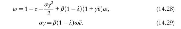
A bit of algebra shows that y is strictly decreasing in τ. Effectively, the tax reduces the value of human capital, ω, which in turn must be associated with a reduction in y (see Equation 14.29). Then, we can see from Equations (14.26) and (14.27) that higher taxes reduce inequality but also reduce the average human capital. This mechanism cap­tures, in stylized form, the idea of Guvenen et al. (2009) used to explain cross-country wage inequality. They argue that higher taxation of labor accounts for the wage com­pression and lower productivity in Europe relative to the United States. Note also that the effects of higher labor taxation in the short run would differ from those in the long run in environments like this. In this particular model, taxation has no short-run disincentive effects (they would exist, however, if leisure were valued). Taxation does have long-run effects because agents would invest less in human capital. Empirical studies based only on short-run data would miss these effects.

14.2.2.2 Human Capital Investment Versus Learning by Doing

The stylized model considered in the previous section can easily be extended to include learning by doing. To do so, we can simply interpret the variable y as the fraction of time spent investing (in human capital) and 1 — y the fraction of time spent producing. Output is produced according to the function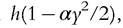which is strictly decreasing and

7

This is in addition to the differences in initial human capital among the I types of newborn agents.

concave in the time spent investing. The equation determining the evolution of human capital becomes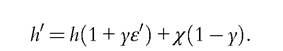

The first term captures the time spent investing, whereas the second results from learning by producing. The analysis conducted so far extends trivially to this case. In particular, the two Equations (14.22) and (14.23) become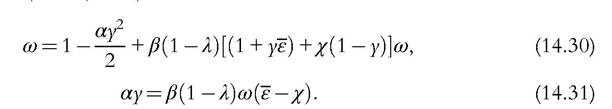

A further extension is to assume that the return from learning by doing is stochastic, that is, χ is a stochastic variable. Also, we could consider the special case in which the evo­lution of human capital is determined only by learning by doing. This case is obtained by setting ε = 0. These extensions do not change the basic properties of the model illustrated in the previous subsection, including the analysis of the short- and long-run effects of labor income taxation.

14.2.2.3 PricesofSkills

So far we have presented a model in which there is only one type of human capital or skills. Individuals have different levels of human capital and, therefore, earn different incomes. In reality, different types of skills are combined together with physical capital to produce goods and services. If those skills are not additive, they have a relative price that may be changing, implying that the distribution of income also depends on those relative prices, which in turn depend on the relative supplies and demands of the various skills.

To fix these ideas, suppose that there are three types of agents according to their skill types, H₁, H₂, and H₃. Production takes place through the technology

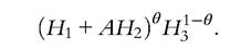
Assuming that markets are competitive, the prices of the three types of skills are equal to their marginal productivities, that is,

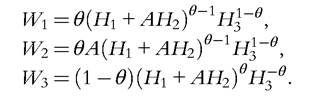
In this example, the relative prices for the three types of skills depend on three factors: (i) the relative supplies of the skill types; (ii) the parameter A determining the productivity of H₂ relative to H₁; (iii) the parameter θ determining the relative productivity between the aggregation of H₁ and H₂ on one side and H₃ on the other. For example, an increase in the parameter A, keeping constant the relative supplies ofthe three skills, increases the productivity of H₂ and H₃ but reduces the marginal productivity of H₁. This changes the distribution of income between the three groups. The change in A could be the result of particular technological progress. As we will see in Section 14.3, a similar idea has been used by Krusell et al. (2000) to explain the increase in the skill premium observed in the United States since 1980.

14.2.2.4 Search and Inequality

Where does workers’ luck come from? Some economists think it is from the arbitrariness of the process that matches workers to jobs. The idea is that some firms are better than others, and these firms end up paying more for essentially identical workers. The argu­ment relies on two considerations. The first is that certain frictions make it difficult for firms to get a worker. The second is that wages depend on the characteristics of both workers and firms.

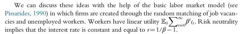
A firm is created by paying a cost κ₀ that entails a draw of a productivity level z from the distribution F(z). After the initial draw, z stays constant over time. Then the firm has to post a vacancy at cost κ₁. If matched with an unemployed worker, the firm produces output z starting in the next period until the match is separated, which happens exog­enously with probability λ. The firm can use only one worker. The number of newly formed matches is determined by the function M(v, u), where v is the number of vacancies and u is the number of unemployed workers. The probability that a vacancy is filled is q = M(v, u)/v, and the probability that an unemployed worker finds occupation is p = M(v, u)/ u. The second ingredient of this model is that wages are determined through Nash bargaining, where we denote by η the bargaining power of workers. A worker attached to a firm with productivity z is paid the wage w(z) and the firm earns z — w(z).

The value of a firm that has a worker can be written recursively as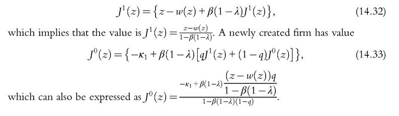

The value of a worker employed by a firm with productivity z is

where U is the value if the worker does not have a job. Such value is given by

where u is the flow utility for the unemployed worker.

To derive the bargaining problem, let’s define the following functions:

These functions are, respectively, the value of a firm and the value of an employed worker, given an arbitrary wage w paid in the current period and future wages deter­mined by the function w(z). The actual wage function w(z) is the solution to the problem Notice that the terms inside the brackets describe, respectively, what the firm and the worker would lose if they do not reach an agreement and break the match. Parameter η captures the bargaining power of workers. To reach an equilibrium, a couple of addi­tional conditions are needed. One is free entry of firms, that is, the expected value of creating a firm,equals its cost, κ₀. To get a steady-state equilibrium, total

firm creation has to be sufficient to create enough vacancies to replace the jobs of workers that join unemployment from job separation.

It is easy to see that the wage is an increasing function of z. In this fashion, a theory of wage inequality can arise from the sheer luck of matching with a very productive firm, even though there is nothing inherently different between two workers in different firms. Hornstein et al. (2011) proposed a new method to assess the quantitative importance of the wage dispersion induced by search frictions and found that it is very small. In fact, the actual dispersion is 20 ? larger than the dispersion generated by the type of search frictions described here. To understand this finding, think of an intermediate step between a worker being matched with a firm and before the actual bargaining process takes place. In this step, the worker could forecast what the wage will be and could potentially choose whether to take the job or keep searching. The minimum wage makes the worker indif­ferent between accepting the job and continuing searching. Such a wage can be com­pared with the average wage that workers get. Hornstein et al. (2011) found that for empirically sound values of the parameters, the difference between the minimum and the average wages generated by search frictions was tiny.

14.2.2.5 Occupational Choice and Earnings Inequality

Workers’ choice of occupation has recently come to the fore as a source of income inequality. Income inequality may occur not only because workers accumulate different levels of human capital, but also because they work in different occupations. As evi­denced by Kambourov and Manovskii (2009b), among others, human capital is largely occupation specific. We will discuss how occupation choices can directly affect the return to human capital and wage growth. In another vein, some workers’ occupations may make them more sensitive to cyclical dynamics and unemployment. As in Wiczer (2013), the occupation specificity of human capital makes workers less flexible in response to specific shocks during the business cycle, and this generates inequality across occupations in terms of unemployment rates, unemployment duration, and earnings.

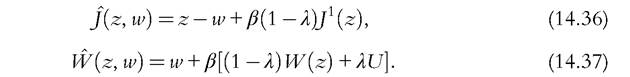
To see the pathways through which occupation choices may affect earnings inequal­ity, consider a simple model with occupations indexed by j = {1,...,J}. Human capital is only imperfectly transferable between occupations. Therefore, the human capital of a worker with current human capital h in occupation j that switches to occupation

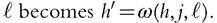
This is the basic framework with which Kambourov and Manovskii (2009a) connected occupational mobility to wage inequality. Workers who remain in the same occupation experience the same wage growth. Workers who switch occupations lose human capital, that is, experience negative growth in earnings. Let’s normalize h = 1 for experienced workers. When a new employee arrives, the human capital is ω_j∕ = ω(1,j,‘), and it takes one period to become experienced. Let g(j,‘) be the prob­ability that a worker switches from j to ‘, and Xj is the measure of workers in occupation j. The variance of wages is

Clearly, without switching occupations, the variance would be zero. But, occupational switching is not infrequent and has, in fact, been rising concurrently with the recent rise in earnings inequality—the probability of switching occupations rose by 19% from the 1970s to the 1990s.⁸ Kambourov and Manovskii (2009a) connect the former to the latter, posing a common cause for both. If occupation-specific shocks are on the rise, they will affect wage inequality through two channels. Directly, they will increase the dispersion in wages of those attached to an occupation, but shocks will also increase switching and create more wage inequality. Because these shocks are difficult to observe directly, Kambourov and Manovskii (2009a) use the occupational switching behavior of workers to inform the underlying process that would generate such behavior; as switching rose,

8

This probability uses the 1970 Census occupations definitions at the three-digit level and PSID data.

the shocks must have also amplified. With this identification logic, occupational switch­ing accounts for 30% of the overall rise in earnings inequality.

Unobserved, occupation-specific shocks are certainly not the only hypothesis for why workers move to different occupations. Several authors, e.g., Papageorgiou (2009) and Yamaguchi (2012), propose that workers’ wages depend on occupation-specific match quality that is learned only through the course of the match. In these papers, earnings inequality is exacerbated by occupational mismatch, which slows the wage growth for some workers. On the other hand, aggregate factors such as business-cycle pressures and unemployment may also increase occupational switching. Indeed, unemployed workers are 3 ? more likely than employed workers to switch occupations. In this vein, we introduce a simple model with unemployment and search as motives to switch occupations.

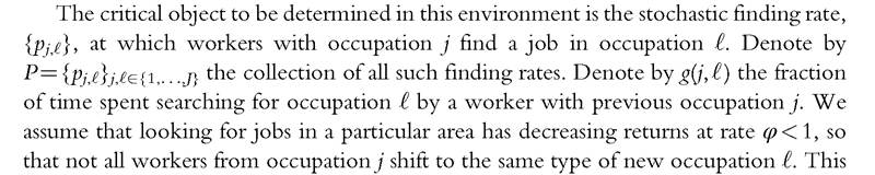
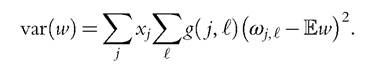
simplification could be a stand-in for any number of more realistic elements of a model such as heterogeneous preferences. Clearly, the allocation of searching time determines the realized finding rate.

The characteristics of the equilibrium are going to depend on the type of wage-setting rule we use, but here we consider the simplest case in which workers earn their marginal product. Hence, the wage of a worker who has just switched occupations is Oj/ and 1 for an experienced worker.

Let W be the value function for an employed worker and U for an unemployed worker. These functions are defined recursively as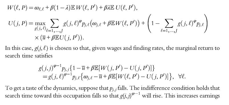

inequality through two channels: (1) the increase in the unemployment rate among type j workers and (2) more of the new matches go to different occupations, where they pro­duce only

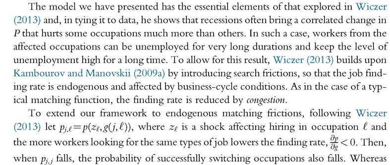
Kambourov and Manovskii (2009a) find their shocks to reconcile switching behavior, Wiczer (2013) maps his shocks to measured value added by occupation. Looking directly at productivity allows Wiczer (2013) to address business cycles in which unemployment and earnings dispersion across occupations increases even though search frictions prevent workers from mass switches into new jobs.

How to identify “occupations” in the data is still an open question. Whereas Wiczer (2013) uses two-digit occupation codes, Carrillo-Tudela and Visschers (2013) take a sim­ilar model but with a finer definition of occupation that highlights the interaction between occupation-specific skills and other job characteristics such as location. Hence, the position of a machinist in Detroit may be even more volatile than machinists in gen­eral. Both papers generate significant volatility in unemployment and earnings over the business cycle beyond search models that abstract from occupational heterogeneity.

14.3.