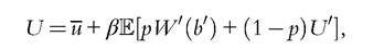
THE DYNAMICS OF INEQUALITY

So far we have looked at how to build theories of inequality in earnings and wealth that aggregate into a macro model. Now we turn to the analysis of factors that affect the dynamics of inequality.

14.3.1 Inequality and the Business Cycle

A well-established feature of the business cycle is that the labor share of income is highly countercyclical. As shown in Figure 14.1, the labor share in the U.S. economy tends to increase during recessions. The figure also shows a declining trend in the labor share since

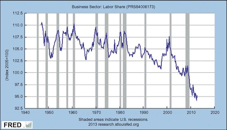
Figure 14.1 Labor share in the U.S. business sector as defined by the Bureau of Labor Statistics. Source: U.S. Department of Labor: Bureau of Labor Statistics.

the early 1980s. To the extent that agents are heterogeneous in the sources of their income—that is, some agents earn primarily capital incomes whereas others earn primar­ily labor income—there is significant redistribution over the business cycle.

To capture the cyclical properties of the labor share, we have to deviate from the stan­dard neoclassical model with a Cobb-Douglas production function, because in this model the labor share is constant. In this section, we review some models in which the compensation of workers is determined through bargaining between employers and workers. Because the bargaining strength of workers depends on macroeconomic conditions, this mechanism has the potential to generate a labor income share that changes over the business cycle.

We start in Section 14.3.1.1 by using the search and matching model developed in Section 14.2.2.4 modified to allow for the study of the determination of the labor share.

14.3.1.1 The Determination of Factor Shares: Productivity Shocks, Bargaining Power Shocks, and Financial Shocks

Consider a version of the search and matching model described in Section 14.2.2.4 (Pissarides, 1987) in which the owners of firms—investors—are distinct from workers, but in which productivity is stochastic and common to all firms. Therefore, z is the same across firms and changes stochastically over time. We will focus on the distribution of income between investors and workers. Both types of agents have the same utility

As before, a firm is created when a posted vacancy is filled by an unemployed worker. A new firm produces output until the match is destroyed exogenously, which happens with probability λ, but now the level of output varies over time. The number of matches is determined by the matching function M(v, u), where v is vacancies and u is unemployed workers. The probability that a vacancy is filled is q = M(v, u)/v, and the probability that an unemployed worker finds a job is p = M(v, u)/u.

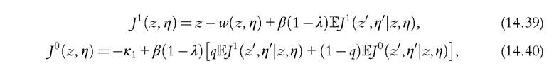
and for workers

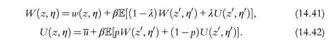
After some rearrangement, the values for the firm and the worker can be written as 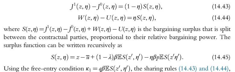and the functions (14.39), (14.41), and (14.42), we can derive the following expression for the wage:

14.3.1.1.1 Shocks to Productivity

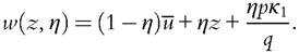
Figure 14.2 plots the impulse responses of employment and the investor’s share of income to a positive productivity shock under the heading baseline model. An economic boom is characterized by a larger share of income going to investors. However, the quantitative effects in terms ofincome distribution and employment are not large. The weak employ­ment response is a well-known property of the matching model (see Costain and Reiter, 2008 or Shimer, 2005). What is interesting is that the inability of the model to generate large employment fluctuations is related to the inability of the model to generate large movements in the distribution of income. Because wages respond too quickly to

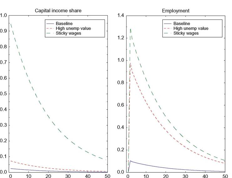
Figure 14.2 Impulse response to productivity shock. The common parameters to all versions of the model are β = 0.985, a = 0.5, Ez = 1, p_z=0.95, σ_z=0.01. The remaining parameters u, ê, l, and A are chosen to achieve the following steady-state targets: a replacement rate of unemployment of 50% (95% in the model with high unemployment value), 10% unemployment rate, 93% probability of filling a vacancy, 70% probability of finding a job.

productivity, the share of income going to investors increases only slightly. As a result, the incentive to create new vacancies does not increase much. However, if wages would respond less, the increase in the share of income going to investors and the increase in employment would be bigger.

Recognizing the direct link between distribution and employment, several authors have proposed some mechanisms for generating smoother responses of wages and, there­fore, larger fluctuations in income shares. Here we summarize three of these approaches. The first approach, proposed by Hagedorn and Manovskii (2008), is to assume that the flow utility received by workers when unemployed is not much smaller than the flow utility from working. In terms of the model, this is obtained by choosing a large value for the parameter U, that is, the flow utility in the unemployment state. Although many consider this assumption implausible, the paper illustrates how this feature could bring the model closer to the data. The second approach proposed by Gertler and Trigari (2009) is to assume that wages are sticky. To illustrate these two cases, we first assign a higher value for the parameter u so that the replacement rate from unemployment is 95%. The impulse responses for this case, plotted in Figure 14.2, are labeled “High unemp. value.” The figure also plots the impulse responses when the wage is exogenously fixed at the steady state with flexible wages (an extreme case of wage rigidity). As can be seen, both assump­tions generate much higher volatility of employment and income distribution between investors and workers. This shows that inequality and macroeconomic volatility are closely interconnected: more volatile income distribution over the business cycle is asso­ciated with greater macroeconomic volatility.

14.3.1.1.2 Shocks to Bargaining Power

Although it has been customary to assume that macroeconomic fluctuations are driven by productivity shocks, economic disturbances have many other possible sources. Here we summarize the effects of shocks that have a direct impact on the distribution of income, in particular, shocks that directly affect the bargaining power of workers, that is, the bargain­ing share η. When η decreases, a larger share of income will go to investors, increasing income inequality. At the same time, as investors appropriate a larger share of the surplus, they have a higher incentive to hire workers, thereby inducing a macroeconomic expan­sion. A similar approach has been studied by Rios-Rull and Santaeulalia-Llopis (2010) in the context of a neoclassical model.

14.3.1.1.3 FinancialShocks

The next step is to show that similar effects to those generated by shocks to bargaining power can be generated by the expansion and contraction of financial markets. The pre­sentation of this case follows Monacelli et al. (2011).

Consider another slight modification of the search and matching model presented earlier, where we allow firms to borrow at the gross rate r. Borrowing, however, is subject to the constraint b' ≤ φEj'(b'), where φ is stochastic. This variable captures the possible changes to the tightness of credit markets.

The firm enters the period with debt b. Given the new debt b' and the wage w, the dividends paid to investors are d = z — w + b'/R — b, where R = (1 + r)/(1 — λ) is the gross interest rate paid by the firm conditional on survival. We assume that, in the event of exit, the firm defaults on the outstanding debt.

The equity value of the firm can be written recursively as

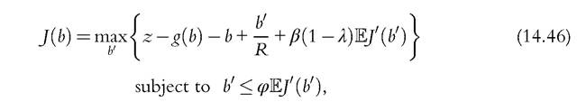
where w = g(b) denotes the (to be determined) wage paid to the worker. As we will see, the wage will depend on the debt. Notice that we have also used a prime to denote the next period value of equity, because this also depends on the next period aggregate states, specifically, the unemployment rate and credit market conditions. To avoid cumbersome notation, we do not include the aggregate states as explicit arguments of the functions defined here. Instead we use the prime to distinguish current versus future functions.

The value of an employed worker is

which is defined once we know the wage g(b). The function U is the value of being unemployed and is defined recursively as

where p is the probability that an unemployed worker finds a job and u is the flow utility for an unemployed worker. Although the value of an employed worker depends on the aggregate states and the individual debt b, the value of being unemployed depends only on the aggregate states, because all firms choose the same level of debt in equilibrium. Thus, if an unemployed worker finds a job in the next period, the value of being employed is W (b').

The determination of the current wage solves the same problem as in Equa­tion (14.38). We should take into account, however, that this solution also depends on b and on the function that determines future wages. Therefore, we write the solution of the bargaining problem as w = ψ(g; b), where g is the function determining future

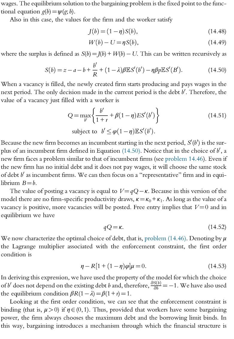
determined (Modigliani and Miller, 1958 does not apply). The reason is clear: by using outside finance, the firm is able to reduce the surplus that is bargained with the worker, increasing the possible rewards to equity.

To gather some intuition about the economic interpretation of the multiplier μ, it will be convenient to rearrange the first order condition as

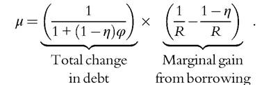
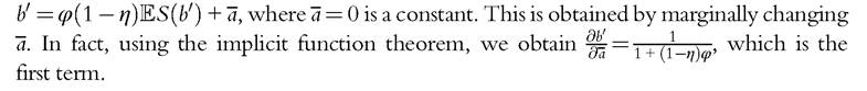
The multiplier results from the product of two terms. The first term is the change in next period liabilities b⁰ allowed by a marginal relaxation of the enforcement constraint, that is,

The second term is the actualized net gain from increasing the next period liabilities b⁰ by one unit (marginal change). If the firm increases b⁰ by one unit, it receives 1/R units of consumption today in the form of additional dividends. In the next period, the firm has to repay one unit. However, the effective cost for the firm is lower than 1, because the higher debt allows the firm to reduce the next period wage by η, that is, the part of the surplus going to the worker. Thus, the effective repayment incurred by the firm is 1 — η. This cost is discounted by R = (1 + r)/(1 — λ) because the debt is repaid only if the match is not separated, which happens with probability 1 — λ. Thus, the multiplier μ is equal to the total change in debt (first term) multiplied by the gain from a marginal increase in borrowing (second term).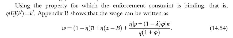

This equation makes clear that the initial debt B acts like a reduction in output in the determination of wages. Instead of getting a fraction η of output, the worker gets a frac­tion η of output “net” of debt. Thus, for a given bargaining power η, the larger the debt the lower the wage received by the worker. This motivates the firm to maximize the debt, as we have already seen from the first order condition.

Figure 14.3 plots the impulse responses to a credit shock, that is, a shock that raises φ and increases the credit available to firms. The credit expansion generates an increase in the capital income share and an increase in employment. Thus, changes in financial markets could alter the distribution of income and, with it, affect the incentives to create jobs. This is another example of how the distribution of income and macroeconomic performance are directly interconnected.

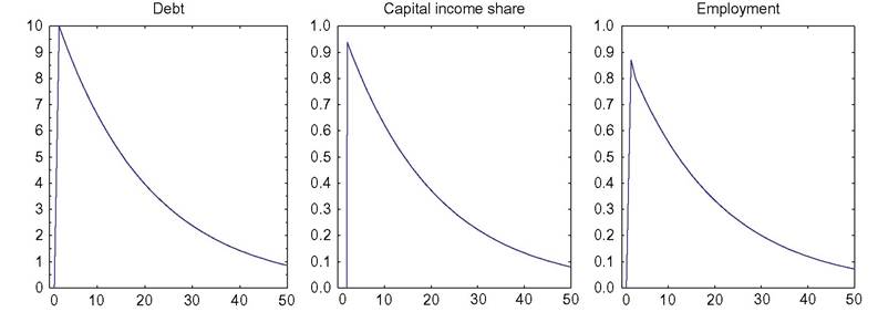
Figure 14.3 Impulse response to credit shock. The parameters are β=0.985, a=0.5, Ez = 1, p_z=0.95, σ_z = 0.01, U = 0.473, ê = 0.316, l = 0.103, and A = 0.807, φ = 0.0022, p_φ = 0.95, σ_φ = 100.

14.3.1.2 Financial Accelerator and Inequality

A well-established tradition in macroeconomics introduces financial market frictions in business-cycle models. The key ingredients are based on two assumptions: market incompleteness and heterogeneity. Although not often emphasized, inequality plays a central role in these models. For example, in the seminal work of Bernanke and Gertler (1989) and (Kiyotaki and Moore (1997), entrepreneurial net worth is central to the amplification of aggregate shocks. When more resources are in the hands of con­strained producers (i.e., these agents are richer), they can expand production and enhance macroeconomic activities. This can happen because they earn higher incomes or because their assets are worth more following asset price appreciations. Thus, these models posit a close connection between profit shares and the business cycle.

These models share some similarities with the matching models reviewed above: when a larger share of output goes to investors/entrepreneurs, the economy expands. At the same time, as the economy expands, a larger share of output or wealth (or both) is allocated to entrepreneurs. The mechanism of transmission, however, is different. In the matching model, the mechanism is the higher profitability of employment or invest­ment. In the financial accelerator model, instead, it is the relaxation of the borrowing constraints. For a detailed review of the most common models used in the literature to explore the importance of financial frictions for macroeconomic fluctuations, see Quadrini (2011).^[16]

14.3.2Low Frequency Movements in Inequality

We discuss here some theoretical ideas that have been proposed in the literature to explain some of the trends in the distribution of income that have occurred since the early 1980s. In Section 14.3.2.1 we look at the reduction in labor share, and in the following two sections we look at the increased inequality in wages and earnings. In Section 14.3.2.2 we examine the potential role of increased competition for human cap­ital and in Section 14.3.2.3 the changes in the prices of skills due to skills-biased technical changes.

14.3.2.1 Labor Share's Reduction Since the Early 1980s

In a recent paper, Karabarbounis and Neiman (2014) document that labor share has sig­nificantly declined since the early 1980s for a majority of countries and industries. They pose a constant elasticity of substitution (CES) production function with nonunitary elas­ticity of substitution between labor and capital and argue that the well-documented decline in the relative price of investment goods (see Cummins and Violante, 2002; Gordon, 1990; Krusell et al., 2000) induced firms to substitute away from labor and toward capital. The consequence was the reduction in the price of labor. They conclude that roughly half of the observed decline in the labor share can be attributed to this mechanism.

To see how this mechanism works, consider the following aggregate production function:

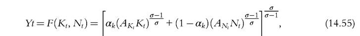
where σ denotes the elasticity of substitution between capital and labor in production, α_k is a distribution parameter, and A_Kt and A_Nt denote, respectively, capital-augmenting and labor-augmenting technology processes. As σ approaches 1, this becomes a Cobb- Douglas production function. Under perfect competition, marginal productivities yield factor prices and one can easily obtain expressions for labor share that crucially depend on the elasticity of substitution σ.

Karabarbounis and Neiman (2014) estimate σ by using only trends in the relative price of investment and the labor share in a cross section of countries. They find a value of 1.25. With this value, the decline in the (observable) relative price of investment accounts for 60% of the observed reduction in labor share. The remaining reduction can be imputed to larger increases in capital-augmenting technology relative to labor-augmenting tech­nology, and to changes in noncompetitive factors (the most important, perhaps, are the permanent changes in the bargaining power of workers relative to firms along the lines of the models discussed earlier). Additional explanations arise from changes in the sectoral composition of output toward industries with higher capital share (which does not really seem to be the case), in part associated with globalization or the increase in the share of output that is traded with other countries, especially developing countries.

14.3.2.2 Increased Wage Inequality: The Role of Competition for Skills

There has been a big increase in earnings dispersion that is well documented in the lit­erature. A glimpse of it can be seen in Tables 14.3 and 14.4. We now explore a possible explanation based on increased competition for skills in the context of human capital accumulation. We have already seen in Section 14.2.2.1 that human capital accumulation could be an important mechanism through which income becomes heterogeneous and that the higher the incentive to invest in human capital, the greater the degree of income inequality. We now look at one of the mechanisms that could affect the incentive to invest in human capital: competition for skills.

To study the importance of competition, we explore yet another version of the matching model described above by adding investment in human capital. We ignore here the possibility of firms to raise debt and limit the analysis to the version of the model with­out aggregate shocks. However, we now assume that output depends on the human cap­ital of the worker, denoted by h. The production technology has a structure similar to the model presented in Section 14.2.2.1. The key feature of the model we look at now is that human capital investment requires both an output loss or pecuniary cost within the firm denoted by y and a utility cost for the worker that we assume quadratic,Given y, human capital evolves stochastically according to

where ε is an i.i.d. random variable. The gross growth rate of human capital is denoted by

Because the outcome of the investment is stochastic, the model generates a complex dis­tribution of human capital among workers. In the long run, the distribution will be degen­erate because at the individual level, h follows a random walk. We assume that workers die with probability λ and that a match breaks down only when a worker dies. Thus, λ represents at the same time the death probability of a worker and the probability of separation of a match. In this way, the distribution becomes stationary and converges to a steady state.

There are contractual frictions that derive from the ability of the worker to control the investment y after bargaining over the wage. The worker unilaterally chooses an invest­ment y that may be, and indeed is, different from the investment that maximizes the sur­plus of the match. This would be the investment that the worker would choose if he had been able to commit. Of course, when the firm bargains the wage, it anticipates the investment that the worker will choose in absence of commitment.

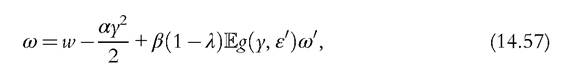
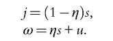
Let’s define a few items. We can write the values of the investor and the worker in normalized form, that is, rescaled by human capital h. Then, the value for the investor can be written as

where j =J/h and w is the wage per unit of human capital. The total wage received by the worker is wh. The value for the worker is

where

The value of being unemployed is

where u = U/h.

Even though in equilibrium, employed workers do not lose their occupation, u is important because it affects the threat value in bargaining. In a steady state we have v = v⁰,

The optimal investment y chosen by the worker maximizes the worker’s value, that is,

with the first order condition given by

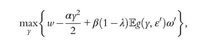
The important part to remember is that bargaining happens before the worker chooses her investment, which means that the surpluses that enter the problem take the invest­ment y as determined by condition (14.59). From this condition we can see that y depends on ω^l but not on the current value of ω, which implies that y is not affected by the outcome of the wage bargaining in the current period. Effectively, the current bargaining problem takes y as given and solves

The first order condition implies that the parties split the net surplus, s =j + ω — u, accord­ing to the bargaining weight η, that is,

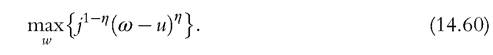
As a comparison, we can also characterize the optimal investment when the worker commits to a particular y chosen to maximize the surplus of the match. In this case, the bargaining problem maximizes the objective (Equation 14.60) over both w and y. The first order condition with respect to w does not change, whereas the first order condition with respect to y becomes

Compared with the optimality condition when the investment is controlled by the worker, Equation (14.59), we observe that the left-hand side and right-hand side terms in Equation (14.61) are both bigger. Therefore, the optimal choice of y with commit­ment could be smaller or bigger. However, provided that α is sufficiently small, that is, the cost for the worker is not too large, the investment without commitment will be bigger.

14.3.2.2.1 General Equilibrium and the Impact of Competition

So far we have not worried about what happens outside the match, but there is a free entry condition that determines how many vacancies are posted. This is given by

where κ is the normalized cost of a vacancy.¹⁰ One way of thinking about increased com­petition is that the entry cost κ is lower. We then have the following proposition.

Proposition 3.1 The degree of competition κ affects the steady-state value of y only in the environment without worker commitment.

This result has a simple intuition: A lower κ is associated with a higher probability that an unemployed worker finds an occupation. As a result, the value of being unemployed increases. Inasmuch as this represents the threat value in bargaining, the worker can extract a higher wage w, which in turn increases the incentive to invest.

We can now show how an increase in competition (lower κ) affects inequality and aggregate outcomes simultaneously. In particular, we have that lower κ generates: (i) more risk taking and greater income inequality and (ii) higher aggregate income. The first effect can be seen from the first order condition (14.59). A lower entry cost increases the number of vacancies and, therefore, the value of finding another occupation if the worker quits. This allows the worker to bargain a higher wage, which in turn increases the employment value ω. We can then see from Equation (14.59) that a higher value of ω is associated with a higher y. As we have seen in Section 14.2.2.1, a higher y implies greater inequality. The second property—the increase in aggregate income—is obvious because a higher y implies higher aggregate human capital. Thus, there is a trade­off between inequality and aggregate income.

Cooley et al. (2012) use a model with similar features but where the accumulation of human capital takes place in the financial sector. They show that greater competition for skills in the financial industry increased the incentive to invest in human capital and gen­erated greater income inequality within and between sectors. This seems consistent with the recent increase in inequality, with income more concentrated at the very top of the

10

For simplicity we are assuming that the cost of vacancies is proportional to the amount of human capital.

distribution and in certain professions, namely, managerial occupations in the financial sector. This pattern is also observed in the United Kingdom, as documented by Bell and Van Reenen (2010).

The idea that competition may increase inequality may go against the common wisdom that wealth is very concentrated because those who control wealth are able to protect it by limiting competition. From this the call is for increased enforcement of competition to reduce inequality. Of course, this does not mean that the theory described above is not valid. It depends on the particular environment we are studying: in certain sectors competition may lead to more inequality, in other sectors to lower inequality.

The degree of competition is just one way of affecting the equilibrium properties of aggregate income and inequality. Taxes are also important. In the context of this model, higher taxes discourage human capital investment (because the after-tax return from investing is lower), but this could be mitigated by the tax deductibility of the investment. Because the costs (curtailment of future earnings) and benefits (tax deductibility) occur at different stages of life when the individual has different incomes, the degree of progres­sivity becomes more important than the overall taxation. However, to the extent that taxes reduce investment, they also lower inequality (because lower investment reduces the volatility of individual incomes).

14.3.2.3 Skill-Biased Technical Change

In addition to increased competition for skills, which ends up rewarding those who are more skilled, a natural explanation for the increased earnings inequality is skill-biased technical change (Katz and Murphy, 1992). Although this term refers in general to changes in the distribution of earnings as a whole, it is often applied more specifically to the premium that college-educated people command compared with those without a college degree. This is motivated by the fact that the college wage premium, defined as the mean log wages of college graduates relative to high school graduates, has increased from 0.3 to 0.6 (see Goldin and Katz, 2009).

To illustrate how skill-biased technical change may have contributed to the increased earnings inequality, consider the following production function:

where S stands for the number of skilled workers (with a college education) and U stands for the number of uneducated workers (without a college education). A_s0 and A_ut are exogenous technical coefficients that could change over time. Under perfect competition in the labor market, wages are marginal productivities, that is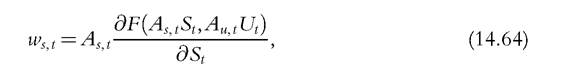

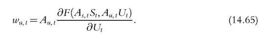
The skill wage premium is defined as

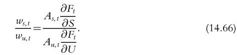
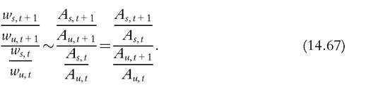
This implies that the increase in the wage premium is owing to faster growth in the tech­nology coefficient A_stt relative to the growth of A_ut, hence, the commonly used term “skill-biased technical change.” But is there something more tangible than just an exog­enous and largely unobserved technological change, or can we track it down to some­thing observable?

Krusell et al. (2000) argued that we can relate these changes to something observable. Gordon (1990) and later Cummins and Violante (2002) have documented that the price of equipment (which is the main part of capital) in terms of consumption goods has gone down dramatically during the period of the rising skill premium. At the same time, the quantity of equipment has gone up significantly relative to output. This is a measurable form of technical change. Combine this with the notion that equipment or capital and skilled labor are complements, whereas unskilled labor is a substitute, and we have an actual channel through which technical progress is skill biased. The formulation in Krusell et al. (2000) does not have factor-specific technical change because all the effects of skill-biased technical change are in the increased quantity of equipment and can be written as

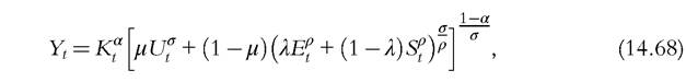
where K_t stands for structures (buildings) that play no role as they enter the production function in a Cobb-Douglas form, U_t and S_t are again unskilled and skilled labor, and E_t is equipment. Using observed measures of inputs, they estimated the elasticities of substi­tution ρ and σ and the share parameters α, λ, and μ, and found that unskilled labor is indeed a substitute for the aggregate of equipment and skilled labor, with both items being complementary to each other. They also found that this specification accounts very well for the observed wage premium under perfect competition for factor inputs.

Other forms of technical innovation indirectly generate skill-biased technical change. Suppose that technical change, regardless of its final effects on total productivity, is some­times more dramatic than other change. The introduction of information technology could be one of these instances even if its impact on productivity is not as clear (Solow, 1987). Yet, the adaptation to this new technology may be easier for educated people. This is the approach taken by Greenwood and Yorukoglu (1974), Caselli (1999), and Galor and Moav (2000). Alternatively, suppose that information technology reduces information and monitoring costs within firms, allowing for reorganizations with fewer vertical layers and with workers performing a wider range of tasks. This gives edu­cated workers an advantage. See, for example, Milgrom and Roberts (1990) and Garicano and Rossi-Hansberg (2004). Yet another form of skilled-biased technical change is an increase in competition for skills, as in the previous section, which could be the result of the technical change. In the context of the model studied earlier, the tech­nical change can take the form of a lower vacancy cost κ. The lower κ increases the demand of skilled workers, which in turn increases the incentive to accumulate skills.

The technological innovations introduced in the 1970s seem to have affected the economy in other respects. Greenwood and Jovanovic (1999) and Hobijn and Jovanovic (2001) assume that new information technologies required a level of restruc­turing that incumbent firms could not face. As a result, their stock market value dropped. This is another form of redistribution in the sense that the owners of incumbent firms lost market value to the owners of new firms. Acemoglu (1998) has proposed a theory of the technical change itself being the result of a surge in college graduates.

The rise of superstars is another possible mechanism that increases the concentration of income. Rosen (1981) viewed the increase in earnings dispersion among people in some occupations as the result of an increase in their ability to reach more users of rare skills. Although this applies naturally to the case of artists and athletes, it also applies more generally to other types of skills. For example, Gabaix and Landier (2008) propose a the­ory of CEO pay where the value of managerial superstars is enhanced by the increase in the size of firms.

14.3.2.3.1 Skill-Biased Technical Change and Human Capital Accumulation

How does human capital investment interact with skill-biased technical change? Heckman et al. (1998) provide an answer that relies on the difference between observed wages and the price of skills that is due to the unpaid on the job investment of the Ben- Porath (1967) type models. They find no special role to capital in generating the increase in the skill wage premium. Instead, they find that the endogenous response of both more college attendance and the allocation of time to invest in further skills is sufficient to account for the patterns in the data. Guvenen and Kuru⅞ςu (2010) also explore the inter­action of skill-biased technical change and human capital accumulation emphasizing dif­ferences across people in the ability to acquire human capital. Guvenen and Kurusςu (2010) argue that increased biased technical change immediately induces an increase in investment by talented individuals that first depresses the skill wage premium and then raises it and that is consistent with the observed bad performance of median wages and with the lack of increase in consumption inequality.

14.4.