INEQUALITY AND FINANCIAL MARKETS

A large body of work links, theoretically, inequality and financial markets. The lack of complete markets helps to shape inequality through two channels. In Section 14.4.1 we study how the limited access to borrowing prevents poor households from undertaking valuable investments.

In the environments studied in the first two sections, the borrowing limits are set exogenously. In Section 14.4.3 we start exploring endogenous theories of the borrowing limit by looking at environments in which the ability to borrow is limited by the incen­tive to default. In doing so, we follow the ideas suggested in Kehoe and Levine (1993). In Section 14.4.4 we review recent papers in which the limits to borrow come from the legal ability to default on debts allowed by the U.S. bankruptcy code. In Section 14.4.5 we explore various extensions of these models. Finally, in Section 14.4.6 we briefly discuss the literature that links the long-term performance of an aggregate economy with the ability of households to borrow.

14.4.1 Financial Markets and Investment Possibilities

Agents with available funds are not necessarily those with the best opportunities to use the funds. It is then socially desirable that the funds are channeled from the former to the latter, which is the primary role played by financial markets. Financial market imperfec­tions, however, limit the volume of funds that can be transferred, and as a result the allocation is inefficient.

Financial market imperfections can take different forms. In a simple overlapping gen­erations model in which the only decision that agents make is how much to invest in the education of their children, the lack of borrowing possibilities implies that investments with a rate of return higher than the risk-free rate will not be undertaken.

To illustrate the importance of financial market frictions, consider an environment in which agents can save but cannot borrow, similar to that of Aiyagari (1994) developed in Section 14.2.1.3.2. The difference now is that the amount of efficiency units of labor is not random but is the result of investment. Consequently, two different investment strategies are available: households can save in the financial asset a (which in this model is backed by real capital), or they can invest in their own human capital so that s⁰ = φ(s, y), where y is the amount invested. The household’s problem can be written as

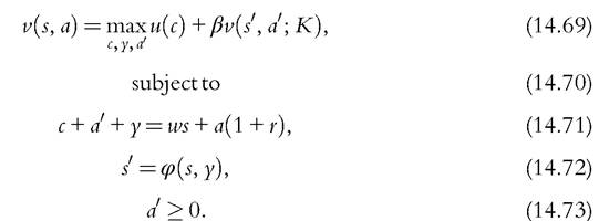
If constraint (14.73) is not binding, the first order conditions of this problem imply

that is, the rate of return of the two types of investment is equalized. Moreover, imagine for simplicity that φ(s, y) = φ(y); then in a steady state, all agents will have the same labor income. An interesting feature of this model is that convergence will arise immediately. That is, all households will have within a period the same labor income, because all agents will make the same investment in human capital. Differences in initial wealth perpetuate. For more general human capital production functions, we can get similar results, with the speed of convergence depending on the decreasing returns in s but not on y.

How would the analysis change when constraint (14.73) is binding? It all depends on the shape of function φ(s, y). Let’s start with the case φ(s, y) = φ(y).

This equation looks very similar to the Euler equation in the standard representative agent growth model, in which there is curvature in the production function. Conse­quently, no matter how poor they start out,all agents will slowly but steadily converge to a level of human capital that satisfies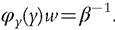So the economy converges to equal

labor income, even if the wealth distribution can be very unequal. Policies that subsidize investment in human capital could speed up the equalization process but will not change the eventual convergence outcome.

A lot of concern remains about poverty traps, that is, situations in which households that start with insufficient initial resources never abandon their poverty status. For this

situation to happen, some special assumptions are needed. In particular, φ(y) cannot be strictly concave. The typical assumption is to have a state of discontinuity such as a min­imum expenditure that is needed to increase human capital. One example is the invest­ment required for educational advancement. In this case, households compare the two options: whether to invest in education or not. If initial household wealth is very low, they may be unable to invest and still have positive consumption. But even house­holds with slightly higher initial wealth may find that educational investment is feasible but not worth it, because it requires that initial consumption is way too low and the cost in utility terms too high. Clearly, in cases like these, government intervention can be fruitful because it is able to circumvent households’ inability to borrow. The government can tax richer households today and transfer resources to the poorer households, or it can borrow, transfer resources to the poor households, and tax them later after they have acquired more education.

Another possibility in which the structure of financial markets matters is to have a stochastic return to the investment technology. Consider a version of Equation (14.72) where higher investments in y yield a high expected value of s⁰ but also a high variance. If the household had access to insurance markets, then it would happily undertake the investment, but if not, its risk aversion would prevent it from doing so. Again, in this case, certain government interventions that provide some form of insurance could be desirable.

14.4.2 Changes in the Borrowing Constraint

One way of assessing the role of financial constraints is to see what happens when they are relaxed. The Aiyagari (1994) model described in Section 14.2.1.3.1 assumes that financial markets are extremely underdeveloped: only one asset needs to be backed by physical capital, and there are no borrowing possibilities. What would happen if the financial con­straints were to be relaxed, that is, what if we allowed for some noncontingent borrowing?

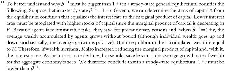
Table 14.7 shows the steady-state wealth distribution under various borrowing limits that go from a quarter of per-household yearly GDP to 1-year GDP. Figure 14.4 shows their associated Lorenz curves. We can see from the figure that, regardless ofthe calibra­tion of the earnings process, inequality increases substantially with the relaxation of the borrowing constraint, in some cases to implausible levels (we cannot imagine an actual economy in which more than 60% of the population have negative financial assets). The Gini indices go up substantially, with one economy displaying a value above one, which is possible when we allow for negative values for the variable of interest. Looser borrow­ing constraints are associated with greater inequality because the poorest households want

Table 14.7 Distribution of wealth for various borrowing limits (in terms of per household yearly output)

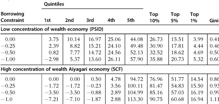
to borrow more.

return of their savings.¹¹ This result creates an incentive to anticipate consumption when the realization of earnings is low, which is made possible by the greater availability of credit (looser borrowing limit). This mechanism generates a greater concentration of wealth, as shown in Figure 14.4 and Table 14.7.

Another possibility is that improvements in the financial market allow agents not only to borrow more but also to buy insurance. In this case, agents could acquire assets or take liabilities with payments contingent on the realizations of idiosyncratic shocks. One

consequence is that households will no longer save for precautionary motives, because they can completely insure their individual consumption. Furthermore, there would not be too much aggregate savings, as in the economy without insurance. So the econ­omy would slowly reduce savings until the interest rate became equal to the rate of time preference. Individual consumption could differ across households, as consumption depends on the initial distribution of physical and human wealth, as in Chatterjee (1994) (see Section 14.2.1.1).

Another important question is, how much borrowing can be sustained? In a model without leisure choice, the maximum sustainable debt is the one that can be paid in all states of nature.

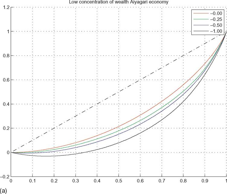
Figure 14.4 Lorenz curves for various economies and borrowing limits. (a) Low concentration of wealth economy (PSID) calibrated as in Aiyagari (1994).

(Continued)

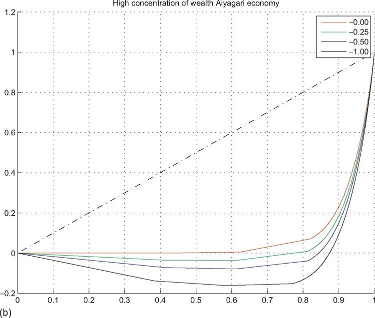
Figure 14.4—Cont'd (b) High concentration of wealth economy (SCF) calibrated as in Castaneda et al. (2003).

is γ, because the interest on this debt is exactly s. Sometimes this is called the solvency constraint. Any debt larger than this value has a positive probability of not being paid.

14.4.3 Limits in the Ability to Borrow

So far, we have considered environments in which the access to credit markets is arbi­trarily limited and there are no markets for contingencies. But why not? What limits the set of contracts that people can sign?

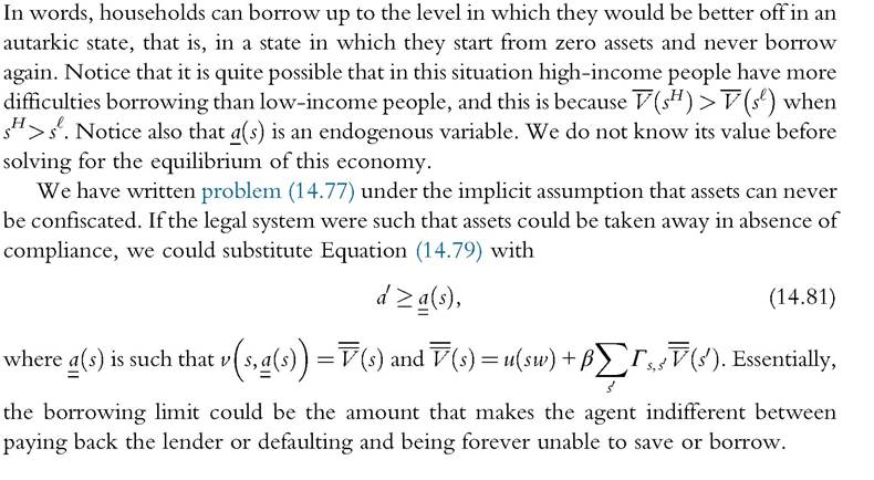
In a well-known and influential paper, Kehoe and Levine (1993) postulated that the ability of households to borrow is limited by their willingness to pay back when the alter­native is to give up access to credit markets. In addition, a subset of the assets (physical or human or both) or endowments of the households can be seized, but not necessarily all of them. For example, future labor income may be outside of the reach of creditors.

Their approach does not preclude the existence of contingent markets. We would like to emphasize two features of this approach. The first feature is that it is the institu­tional environment that determines the set of contracts that are available. We think that this is an enormous advance compared with the literature that relies on exogenous bor­rowing limits. The second feature is that only the contracts that can be enforced ex post are available in the market. Therefore, once signed, there is complete compliance in the execution of these contracts. This feature is perhaps less appealing, as we see actual ex post reneging on formal contracts.

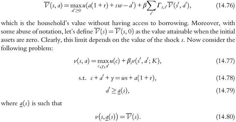
To show how this works, we could again slightly modify the Aiyagari economy. Let’s first define the following object:

In this model, all contracts are carried out, that is, loans and state-contingent contracts are always honored. In reality, however, many people file for bankruptcy. For example, in the 12 months between April 1, 2012, and March 31, 2013, 779,306 people filed for bankruptcy in the United States.¹² In some countries including the United States and Canada, debts are typically discharged after filing, whereas in other countries, such as Hungary, Romania, and Spain, there is no legal procedure to handle personal bank­ruptcy, and people are always liable for previous debts. The rest of the countries lie some­where in between these extremes.

One possible strategy to deal with the pervasiveness of bankruptcy is to model it as a contingency fully negotiated ex ante by the parties. This strategy is hard to justify, how­ever, because filing for bankruptcy is a legal procedure that can be completed unilaterally by the debtor. Hence, it is a right that cannot be forfeited. We need, then, to have explicit models that explicitly incorporate bankruptcy filings. One approach, followed within the optimal contracting tradition, is to assume that there are information asymmetries and costly state verification, as in Townsend (1979). The costly state verification model has been widely applied in macroeconomics, for example, in Bernanke and Gertler (1989), Bernanke et al. (1999), and Carlstrom and Fuerst (1995). In these models, default arises in equilibrium even if agents sign fully optimal contracts. In the next section, we will describe other approaches that are more in line with the literature that excludes the applicability of fully optimal contracts.

14.4.4 Endogenous Financial Markets Under Actual Bankruptcy Laws During the last few years, considerable work has been done to bring together models with imperfect insurance and models with a legal system that allows agents to file for bank­ruptcy in a way that is similar to that of Chapter 7 in the U.S. bankruptcy code (Chatterjee et al., 2007; Livshits et al., 2007). We now present a version of these models and describe how their implications for the income and wealth distribution change com­pared with the basic Aiyagari model. These studies take advantage of a feature of the legal system that lists people who have filed for bankruptcy in public records for a certain num­ber of years. The literature interprets the implications of the listing as limiting accessibility to borrowing for the duration of the public record.

Consider the following household problem, yet another variant of the basic Aiyagari problem: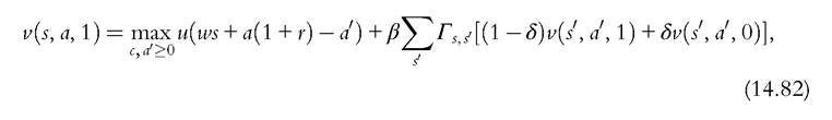

12

See U.S. courts, http://www.uscourts.gov/.

The function v(s, a, h) is the household’s value function, with the last argument h 2 {0,1} denoting the household’s credit history. When h = 1, the household’s credit history is bad in the sense that the agent has defaulted in the near past and is prevented from having access to credit. Problem (14.82) depicts this case, showing that in the following period, its credit history may turn out to be good, h = 0, with parameter δ controlling the expected duration of market exclusion.

Problem (14.83) is of interest when the credit history is good, h = 0, and we have written it compactly, implicitly assuming that the household is in debt, a < 0. Here, the agent has two options: to file for bankruptcy or not. If the agent files, three things happen: household consumption equals current labor income, sw, credit history turns bad next period, h⁰ = 1, and the household is prevented from saving. The latter property is a feature of the bankruptcy code, as the agent is not permitted to keep assets after filing for bankruptcy. ³ If the household does not file for bankruptcy, it can borrow or save as it wishes. Note, however, that we have written the budget constraint (14.84) differently from previous problems. The left-hand side, the uses of funds, has the asset position at the beginning of the following period multiplied by q(s, α⁰). This is the household-specific inverse of the interest rate. Lenders accurately forecast that the agent may file for bank­ruptcy and charge an extra premium so that in expected value they get the market return. The functionis an equilibrium object. If the household chooses to save, α⁰ ≥ 0, and the inverse of the interest rate is that of the safe asset:

The optimal solution to the problem of a household with negative assets is to default for a range of its earnings. The set of earnings for which the household defaults increases with the stock of debt.

The solution to this problem has two interesting properties. First, inasmuch as default is costly (the household will not be able to borrow for a while), the household would not default if the debt is very small. Second, in some circumstances, the household may be too poor to default, opting instead to borrow even more for a sufficiently low realization of earnings. Consequently, the equilibrium of this model requires that the inverse of the interest rate q(s, α⁰) is such that lenders break even in expected value, which in turn implies that interest rates are increasing in the amount borrowed and in the likelihood of bad earnings realizations.

¹³ In the United States, the agent can keep a maximum amount of assets, and this amount varies across states. Here, we have assumed zero retainable. In the discussion from which we are abstracting are other sub­tleties of the bankruptcy code, such as the requirement that labor income is below the state median’s income.

This structure has proved useful in making sense simultaneously of the extent of unse­cured borrowing in the United States as well as the frequency of bankruptcy filings, espe­cially if the model is enhanced with a few bells and whistles such as expenditure shocks.

14.4.4.1 A Weakness of This Approach

Why are households refused credit when they have a bad credit history? Nothing in the law requires this. In fact, the opposite is true: in the United States, a bankruptcy filing under Chapter 7, the relevant case, precludes additional filings over a period of years, making a recent filer appear to be a better creditor than somebody with a clean slate.

This question has three possible answers, but none are completely satisfactory. First, a Nash equilibrium with a coordination problem can be constructed when lenders believe that agents with bad credit histories will not pay back and hence they will not lend, whereas prospective borrowers might as well choose to default, because they do not receive credit. Although this is indeed a Nash equilibrium, it is one that is always present in the event of lending, and there is no argument for why it happens only with a bad credit history. Another possibility is to construct a trigger strategy whereby lenders coor­dinate not to lend during a punishment period in the event of default. But like all triggers, this is not an equilibrium of the limit of finite economies. Hence, it is not a Markov equi­librium. Many economists are comfortable with trigger strategy equilibria, whereas others are not. The last rationale for exclusion of those with bad credit is to postulate the existence of a regulator that prevents lenders from lending to those with bad credit, something that is not actually done by any of the banking regulators.

14.4.4 Credit Scoring

Chatterjee et al. (2008) and Chatterjee et al. (2004) propose a solution to the weakness of models based on exogenous exclusion after bankruptcy filings. These papers note that in the United States, there is pervasive use of credit scores, which are assessments of reli­ability made by independent companies. The authors then pose a model in which two types of people differ in some fundamental attribute associated with reliability that is not directly observable by outsiders—for instance, patience or even good driving habits. The credit score is then used as the market assessment of being a good type, mean­ing the type that is more likely to pay back debts or be reliable. In this context, both types of agents fall under the model of borrowing in which there are multiple types. The key here is that both types of agents—both the patient and the impatient agents—want to repay their debts to signal that they are patient, which allows them to have access to better borrowing terms. In this context, filing for bankruptcy increases the market-assessed like­lihood that an agent is of the bad type, which translates to a severe worsening of loan terms, if not an outright exclusion of future credit. Moreover, because the market is assessing traits that are relevant not only for the repayment of credit but also for other things (e.g., cheap property insurance, access to rental property, personal relationships), timely repayment of debts carries a strong incentive that allows for the possibility of many contracts to be carried out, even if the law lacks the necessary teeth to enforce these contracts.

14.4.5 Financial Development and Long-Run Dynamics

We now look at the extent to which access to financial markets can help us to understand the long-run dynamics of the economy. In Section 14.4.6.1 we briefly focus on long­term growth, and in Section 14.4.6.2 we discuss how the evolution of financial markets can also help us understand the issue of global imbalances, that is, the emergence of large and persistent balance of payments deficits.

14.4.6.1 Long-Run Growth and Financial Development

The Schumpeterian view places entrepreneurship at the center stage of economic devel­opment. Owing to financial constraints and the lack of insurance markets, however, entrepreneurial investment is suboptimal. Essentially, when financial markets are not well developed, resources cannot be redistributed from those who control the resources but do not have the best uses of these resources to those who have the best investment oppor­tunities but lack the funds. This efficiency problem is especially severe when the distri­bution of resources is particularly concentrated. We may then end up with a situation in which the poor become (relatively) poorer because they cannot take advantage of invest­ment opportunities and the economy as a whole grows less. Examples of studies that emphasize the importance of inequality for growth in the presence of financial constraints are Galor and Zeira (1993), Banerjee and Newman (1993), and Aghion and Bolton (1997). Because these studies were already reviewed by Bertola (2000) in a previous edi­tion of the Handbook, we do not repeat their description in this chapter.

A more recent literature, however, also emphasizes that market incompleteness—that is, environments in which the trade of state-contingent claims is limited—could have both positive and negative effects on capital accumulation. In a world with only unin- surable and exogenous earning shocks as in Aiyagari (1994), market incompleteness gen­erates more capital accumulation and, therefore, more growth. When risky income is endogenous, however, as in Angeletos (2007), market incompleteness may discourage investment. See also Meh and Quadrini (2006).

Another group of studies that investigates the relation between inequality and mac­roeconomic performance emphasizes the importance of social conflict and expropriation. Greater inequality often associated with underdeveloped financial markets means that a larger group of individuals are at the bottom of the distribution and face poor economic conditions compared with the rest of the population. Faced with poor economic con­ditions and the feeling that the prospects for economic improvement are impaired by the excessive concentration of wealth, the resentment toward the rich starts to rise, which creates incentives to expropriate either by stealing or through revolutions. The risk of expropriation has two negative effects. First, it acts as an investment tax that discourages investment. Second, agents devote more resources to protect property rights instead of using the resources for productive and growth-enhancing activities. Benhabib and Rustichini (1996) develop a model that formalizes this idea. Although not explicitly con­sidered in this paper, financial underdevelopment could contribute to this because it makes it more difficult for poor people to escape from poverty.

Another theory of inequality affecting growth is developed in Murphy et al. (1989). This paper assumes that some technologies have increasing returns. These technologies become profitable only if the domestic market is sufficiently large, that is, enough demand exists for the goods produced with the new technologies. Ifwealth is highly con­centrated, the domestic market remains small (because not enough consumers can afford these goods). As a result, growth-enhancing technologies will not be implemented. The paper does not explicitly explore the role of financial markets; however, to the extent that financial underdevelopment creates the conditions for greater concentration of wealth, the mechanism described in this paper becomes more relevant in economies in which the financial structure is relatively underdeveloped.

Kumhof and Ranciere (2010) have proposed an explanation for the recent crisis based on the changes in income distribution pinpointing similarity with the Great Depression. The idea is that, because of an exogenous shock that affected the ability of the rich to grab earnings, income became more concentrated, and as a result, the poor started to borrow more, increasing the debt-to-income ratio in the economy. Eventually, the increase in borrowing triggered the crisis.

We conclude this section by citing the work of Greenwood and Jovanovic (1990). Although this paper does not deal directly with inequality, it shows that improvements in financial markets (in this particular case, through the information gathered by financial intermediaries) have important effects on economic growth. As we have seen in previous chapters, market incompleteness also creates inequality. Therefore, once complemented with the previous analysis, this paper could also be relevant for understanding the link between financial market development, inequality, and growth. Also important is the work of Greenwood et al. (2010).

14.4.6.2 Global Imbalances

We have not talked much about cross-country inequality because this topic is usually a concern for development-oriented economists. However, inequality may be shaped by the increase in trade that is properly known as globalization, which is due to the reduction in the trade barriers for both technological and policy reasons. We have already referred, if only obliquely, to a mechanism by which more trade across countries could affect inequality: opening to trade changes the relative price of skills and may be behind part of the recent increase in the wage-skill gap. But an increase in trade shapes inequality both within and between countries through other, more subtle mechanisms. In this section we illustrate some potential mechanisms through which inequality is linked to globalization. Further analysis of the role of globalization for inequality is conducted in Chapter 20.

The process of international globalization is commonly presented as taking the form of higher trade in goods and services (imports and exports) as a fraction of GDP. But there is another side to it. Several advanced countries, the United States in particular, have experi­enced over the last 30 years a persistent deficit in the balance ofpayments as a result of imports being higher than exports, with the consequent deterioration in their net foreign asset posi­tions. On the other hand, oil-producing countries and several emerging countries, China in particular, have been accumulating positive net foreign asset positions. “Global imbalances” is the term often used to refer to the situation in which some countries accumulate large negative net foreign asset positions whereas others accumulate positive net foreign asset posi­tions. This situation has affected inequality, but to understand the impact on inequality we first need a theory of why imbalances could emerge in the wave of globalization.

Mendoza et al. (2007) provide one such theory. They claim that sustained deficits cannot be explained solely with traditional trade forces (different factor prices, techno­logical advantages, or lower transportation costs). We also need to understand the differ­ential saving behavior of countries that in equilibrium lead to different rates of returns on savings (insofar as international financial markets are somewhat segmented). This is pos­sible even if countries have identical preferences and production technologies, but agents in each country differ in the extent to which they are capable of insuring their individual risks. This can be illustrated with the now familiar Aiyagari economy.

Suppose that we compare two economies, both slightly modified versions of the Aiyagari environment described above, that differ only in the process for earnings, one being more volatile than the other. It is important to point out that the assumption that countries differ in the volatility of earnings is a shortcut to capture other, more micro-founded differences. For example, in Mendoza et al. (2007), countries do not dif­fer in the underlying process for earnings but in the sophistication of financial markets. Agents (consumers and firms) in countries with more advanced financial markets have a better opportunity to insure their idiosyncratic risk. Because in terms of savings the impli­cation of higher insurance is similar to lower variability of earnings, here we illustrate the mechanism by assuming lower earning volatility. In some applications the higher ability to insure could derive from government policies (for example, the provision of public- funded health insurance). In some cases, the differences could come from more uncer­tainty about the underlying process for earnings. For example, a country that is experiencing a process of transformation (such as China, during the last three decades) is also possibly characterized by greater uncertainty at the individual level. Independently of the actual sources (greater ability to insure or greater underlying uncertainty), it should be clear that the example provided here is just a shortcut to illustrate something more fundamental such as differences in the characteristics of the financial system.^[17]

14

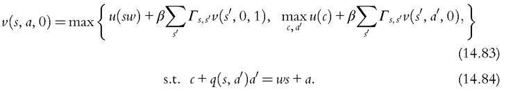
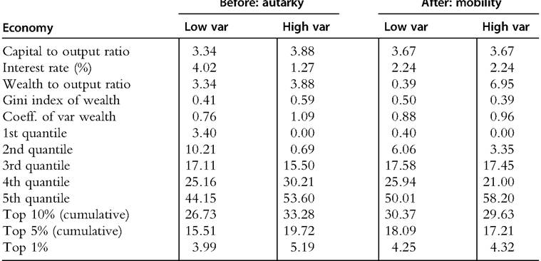
Table 14.8 Two economies before and after being able to borrow from each other

To this end, we use two different processes for earnings. The first process is what we used above for the version of the model that we called PSID economy or low-variability economy. The second process is what we used in the high-variability economy, a version of the SCF economy with a slightly less extreme good state. Besides the process for earn­ings, the two economies are alike in all other dimensions.

The first two columns of Table 14.8 display the steady states of these two economies under autarky. The first column, the low-variability economy, has a capital-to-output ratio of 3.34, implying an annual interest rate of 4.02%. Because in this economy wealth can only take the form of capital, total wealth is also 3.34 ? output, and this is what house­holds choose to hold to accommodate the shocks to earnings given the 4.02% interest rate. The second column of Table 14.8 refers to the economy with higher income variability also in the autarky regime. Households choose to hold more wealth (3.88 ? output) to bear the high risk. Two things to note are that the interest rate is now much lower, 1.27%, and that output is slightly higher because of the higher capital.

The determination of the equilibrium is depicted in panel (a) of Figure 14.5. This figure plots the aggregate (steady-state) supply of savings as an increasing, concave func­tion of the interest rate.^[18] The demand for savings is downward sloping because of the diminishing marginal productivity of capital. Country 1 has a lower volatility of

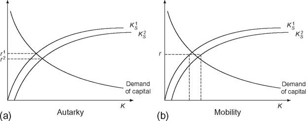
Figure 14.5 Steady-state equilibria with heterogeneous earning risks.

individual earnings and hence a lower supply of savings for each interest rate. As a result, the equilibrium in autarky implies a higher interest rate and a lower total capital.

Imagine now that households in these two economies can start owning capital in the other country, that is, the countries become financially integrated. After a brief period of transition that depends on the ease with which physical capital can flow or be reallocated, the interest rate in both countries will be equalized. This implies that the low-variability economy will experience a reduction in the interest rate and the high-variability econ­omy will experience an increase in the interest rate. Then, in the country in which the interest rate decreases (low-variability economy), savings will fall, whereas in the country in which the interest rate increases (high-variability economy), savings will rise. The result is that households in the high-variability economy end up owning part of the cap­ital installed in the low-variability economy. In this way, global imbalances may emerge as the low-variability economy dis-saves. Effectively, the low-variability economy con­sumes and invests more than it produces, with the difference covered by imports in excess of exports (trade deficit).

This process takes a long time until the aggregate savings of households in each coun­try no longer change. This new steady state is depicted in panel (b) of Figure 14.5. The world interest rate is somewhere between the pre-liberalization interest rates in the two countries. Comparedwith autarky, the interest rate and the supply of savings fall in coun­try 1 and rise in country 2, and hence the country with lower volatility of earnings ends up with a negative foreign asset position. Moreover, the capital stock rises relative to its autarky level in country 1 and falls in country 2. Thus, financial globalization leads capital to flow from economies with more risk to those with lower risk.

For analytical simplicity, we have modeled this process as the outcome of countries that differ in their earnings risk. However, as emphasized above, this is just a shortcut to capture other types of differences across countries that ultimately lead to different expo­sure to risk. It could very well be the case that the underlying risk is identical across coun­tries but that the lower risk in one country is just the result of more-developed financial markets, which allow for higher insurability of risk. Formally, in the first country there are more markets for state-contingent claims. This is the approach taken in Mendoza et al. (2007), and the end result is similar to the case of differential processes for earnings: the country with a higher ability to insure saves less and has a higher interest rate than the country with less-developed financial markets. When the two countries integrate, it is the more financially developed country that accumulates negative foreign assets, whereas the less financially developed country accumulates positive foreign assets.

Therefore, financial market differences can affect the distribution of wealth across countries: in the long run, countries that are more financially sophisticated become poorer relative to countries that are less financially sophisticated (compared to the pre-liberalization era). This, however, does not mean that liberalization is welfare reduc­ing for developed countries and welfare improving for less-developed countries. In Mendoza et al. (2007) we found, somewhat surprisingly, that liberalization was welfare improving for developed countries but slightly welfare reducing for less-developed coun­tries (based on an equally weighted welfare function). In our example displayed in Table 14.8, the international redistribution of wealth is quite large, with the low- variability country ending up with barely 5% of total wealth. Yet, it started with almost half. The large international redistribution of wealth follows from the assumption that there are large differences in risk between the two countries. In reality, especially among integrated countries, the differences in risk may not be that big. Also, when a country accumulates too many foreign liabilities, there could be an incentive to default on these liabilities. This imposes a limit on the redistribution of wealth that can be generated across countries through this mechanism. Nevertheless, this example suggests that differences in savings could generate significant inequality in wealth across countries.

Cross-country financial market heterogeneity also plays a central role in Caballero et al. (2008) for explaining global imbalances. The mechanism proposed in this paper does not rely on risk but on the availability of saving instruments. The idea is that in cer­tain countries, savers have difficulty storing their savings in high return assets. The impli­cations for global imbalances, however, are similar to Mendoza et al. (2007). The two mechanisms are complementary ways of thinking about how the characteristics of finan­cial systems can shape the distribution of wealth across countries in a globalized world. Interestingly, these contributions illustrate another mechanism through which financial globalization redistributes wealth. When productive inputs are not perfectly reproducible (as in the case of land), liberalization also leads to the equalization in the prices of these assets. Because under autarky these assets were cheaper in financially developed countries, these countries experience capital gains, whereas countries with less-developed financial markets experience capital losses.

The process of international redistribution of wealth also has consequences for the internal wealth distribution within each country. We see how wealth concentration increases in the low-variability country as measured by either the Gini index of the coefficient of variation of wealth or even by the shares held by the richest households (see Table 14.8). The opposite process happens in the less financially developed country, where the wealth distribution becomes more equal after international financial integra­tion. Perhaps this process has contributed, at least in part, to the increased wealth con­centration in the United States that we documented earlier.

14.5.