SOME FACTS ON THE INCOME AND WEALTH DISTRIBUTION
Here we outline some general features of the Lorenz curves for earnings and wealth and their correlation and persistence over a medium span of 5—10 years for both individuals and across generations.
We draw data from Diaz-Gimenez et al. (2011), Kuhn (2014), and Budria et al. (2001) for the United States.[11] The data come from the Survey of Consumer Finances (SCF). Although the facts are for the U.S. economy, they may apply in varying degrees to other countries. In general, the United States is a more extreme version of the other developed countries in the sense that it is characterized by higher inequality.Table 14.1 shows the shares of earnings (the part of the income that can be attributed to labor), income (earnings plus capital income plus government transfers before taxes), and wealth (both financial and real assets, but not defined benefits pensions). See Dlaz- Gimenez et al. (2011) for details about the definition of these variables. As we can see, a large number of households have zero or negative earnings, almost two-thirds of all earnings come from the top quintile, and the top 1% receive almost 20% of all earnings. Our definition of earnings includes part of self-employment income that is imputed as labor income.[12] Because self-employment income can be negative, several households have zero or even negative earnings in our sample. Negative earnings contribute to a much higher Gini index compared to other measures provided in the literature, such as those that result from using earnings data from the Current Population Survey (CPS). However, correcting the CPS data by tax information could lead to Gini indexes that exceed 0.6 (see Alvaredo, 2011 and the discussion in Chapter 9). Wealth is more concentrated than income, and the poorest quintile holds negative wealth. Furthermore, more than 85% of the wealth is held by the richest quintile and more than one-third of all wealth by the richest 1%.
Table 14.2 shows a few measures of dispersion that are useful to keep in mind.The properties of the distribution of earnings, income, and wealth (total (Wea) and excluding housing (N-H-W)) have changedin the last few years. Tables 14.3-14.5 show the values of a few measures of concentration for 1998, 2007, and 2010. For earnings, the Ginis, the coefficient of variations, the various ratios involving the median and the shares of top groups have all increased, most of them monotonically. For income, the picture presented by the SCF is muddier. The Gini seems unchanged, with some measures indicating an increase in inequality and others a decrease. The same seems to have happened for wealth. While the Gini, the ratio of the 90th percentile to the median and of the
Table 14.1 Distribution of earnings and net worth in the U.S. economy
| Bottom (%) | Quintiles | Top (%) | All | ||||
| 0-1 | 1-5 5-10 | 1st | 2nd 3rd 4th | 5th | 90-95 | 95-99 99-100 | 0-100 |
Shares of total sample sorted by earnings (%)
| Earnings | -0.1 | 0 | 0 | -0.1 | 3.5 | 11 | 20.6 | 65.0 | 12.1 | 18.3 | 18.0 | 100 |
| Income | 0.8 | 0.4 | 0.9 | 6.5 | 8.5 | 10.5 | 17.8 | 56.7 | 10.3 | 16.5 | 15.9 | 100 |
| Net worth | 4.5 | 0.5 | 0.7 | 11.6 | 13 | 6.3 | 9.9 | 59.1 | 8.6 | 21.2 | 20.2 | 100 |
Shares of total sample sorted by net worth (%)
| Earnings | 0.9 | 2.8 | 2.3 | 8.4 | 10.7 | 14.6 | 17.5 | 48.8 | 10.3 | 15.7 | 10.8 | 100.0 |
| Income | 0.8 | 2.6 | 2.2 | 8.4 | 10.0 | 13.9 | 17.6 | 50.1 | 10.2 | 15.3 | 12.2 | 100.0 |
| Net worth | -0.3 | -0.3 | -0.1 | -0.7 | 0.7 | 3.3 | 10.0 | 86.7 | 13.5 | 26.8 | 34.1 | 100.0 |
Data are from the 2010 Survey ofConsumer Finances. Income includes all transfers including food stamps.
Earnings are defined as the part of income earned by labor. Farm and business incomes are assigned split between labor (93.4%) and capital (6.6%) (a much lower capital share than in other years).Source: Kuhn (2014).
Table 14.2 Concentration and skewness of the distributions for 2010
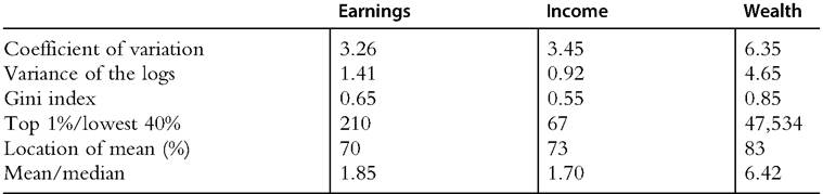
Source: Kuhn (2014).
Table 14 3 Chanes in concentration
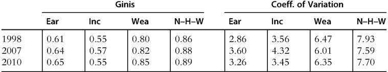
Source: Kuhn (2014).
Table 14.4 Changes of relevant ratios involving the medians
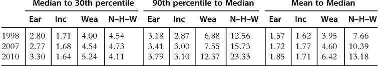
Source: Kuhn (2014).
Table 14.5 Percentages of Total Earnings, Income, and Wealth of Selected Groups
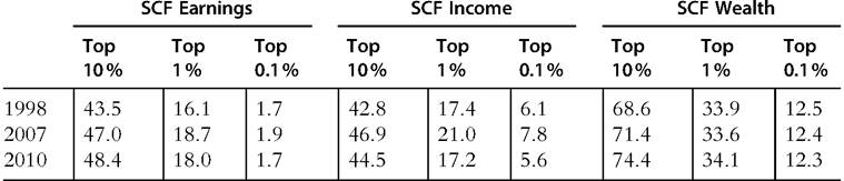
Source: Kuhn (2014).
mean to the median have all gone up, the shares of the top 10%, 1% and 0.1%, have either remained stable or have gone down.
The modest evidence for an increase in inequality in income and wealth contrasts drastically with the picture reported by Piketty and Saez (2003), Piketty (2014), and Saez and Zucman (2014), who have used tax data. They have documented a big increase in inequality in the last few years in both income and wealth. Their evidence for income is direct as it comes straight from tax returns. The evidence for the evolution of wealth concentration in Saez and Zucman (2014) is indirect; it imputes the value of the assets that generate the reported capital income using the capitalization method with the rates of return for each class of assets that are obtained in the Flow of Funds. Yet it is quite persuasive. They suggest that the discrepancies that result between using the SCF and using tax data is due mostly to the top 0.1% of the top wealth holders. The SCF excludes the richest 400 households (the Forbes 400), and it is quite possible that even within income strata, response rates to the SCF voluntary questionnaire vary by income.
The two sets of data are complementary, and the SCF is working hard to improve how it represents the very richest. There is likely to be a major update of the SCF that tries hard to improve in these dimensions. Hopefully, such improvements in the SCF will be available in the next few months, and we will get a much better picture of the characteristics of the very rich.Turning to consumption inequality, there are some doubts about whether it has also increased. Using data from the Consumer Expenditure Survey, Krueger and Perri (2006) have documented that consumption inequality has increased only slightly. However, Attanasio et al. (2004) and Aguiar and Bils (2011) claim that the increase in consumption inequality has been more significant. One of the reasons these studies reach different conclusions is because they use different survey data. Krueger and Perri (2006) use data in which consumption comes from survey collecting interviews, and Attanasio et al. (2004) use diary data. In addition, Aguiar and Bils (2011) have argued that the observed reduction in the quality of the consumption data in terms of how much of aggregate consumption is recovered in the interviews is concentrated among goods that are mostly purchased by rich people and among the high income groups, and both features point to a larger increase in the underlying consumption inequality than what is obtained by using the data without special adjustments.
To summarize, over the last 10—20 years, the evidence points to a sizable increase in inequality.
14.2.
More on the topic SOME FACTS ON THE INCOME AND WEALTH DISTRIBUTION:
- Atkinson Anthony, Bourguignon François. Handbook of Income Distribution. Volume 2B. North Holland, 2014. — 2366 p.,
- SUMMARY AND CONCLUDING REMARKS
- INTRODUCTION
- TAKING ECONOMIC THEORY SERIOUSLY
- CONCLUSION
- INTRODUCTION
- INTRODUCTION
- The Agenda
- CONCLUDING REMARKS
- Abstract