INTRODUCTION

This chapter is about the techniques, formal and informal, that are commonly used to give quantitative answers in the field of distributional analysis—covering subjects such as inequality, poverty, and the modeling of income distributions.

At first sight, this might not appear to be the most exciting of topics. Discussing statis­tical and econometric techniques could appear to be purely secondary to the important questions in distributional analysis. However, this is not so. At a very basic level, without data what could be done? Clearly if there were a complete dearth of quantitative informa­tion about income and wealth distributions, we could still talk about inequality, poverty, and principles of economic justice. But theories of inequality and of social welfare would stay as theories without practical content. Knowing how to use empirical evidence in an appropriate manner is essential to the discourse about the welfare economics of income distribution and to the formulation of policy. Furthermore, understanding the nature and the limitations of the data that are available—or that may become available—may help to shape one’s understanding of quite deep points about economic inequality and related topics; good practice in quantitative analysis can foster the develop­ment of good theory.

6.1.1 WhyStatisticalMethods?

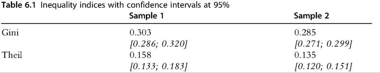
If we carry out a simple computation of the values of an inequality or poverty measure, computed from two different samples, we will usually find greater inequality or poverty in one sample, even if the two samples come from the same population. Clearly simple compu­tation alone is not enough to draw useful conclusions from the raw data: Statistical methods are required to test the hypothesis that the two values are not statistically dif­ferent. For instance, Table 6.1 reports the values of the Gini and Theil inequality indices,¹ with confidence intervals at 95%, computed from two samples of 1000 obser­vations drawn from the same distribution: The two samples are independent, with obser­vations drawn independently from the Singh-Maddala distribution with parameters a = 2.8, b = 0.193, and q = 1.7, which closely mimics the net income of German house­holds, up to a scale factor (Brachmann et al., 1996).

There is a wide variety of inequality indices in common use. Different indices, with different properties, could lead to opposite conclusions in practice. Lorenz curves com­parisons can be very useful because a (relative) Lorenz curve always lying above another one implies that any comparisons of relative inequality measures would lead to similar conclusions—a result that holds for any inequality measures respecting anonymity, scale invariance, replication invariance, and the transfer principle (Atkinson, 1970). In prac­tice, we have on hand a finite number of observations, and empirical Lorenz dominance can be observed many times when the two samples come from the same population. In the case of two independent samples of 1000 observations drawn from the same Singh- Maddala distribution, we obtain sample Lorenz dominance 22% of cases. Dardanoni and Forcina (1999) argued that it can be as high as 50% of cases due to the fact that empir­ical Lorenz curve ordinates are typically strongly correlated. This demonstrates the need to use statistical methods.

The point about simple computation being insufficient is also easily demonstrated in the case of Lorenz curves: Figure 6.1 shows the difference between the empirical Lorenz curves obtained from two independent samples drawn from the same distribution, with confidence intervals at 95% calculated at the population proportions q = 0.01, 0.02,..., 0.99. The ordinates are always positive, so it is clear that one empirical Lorenz curve always dominates the other. However, the confidence intervals show that each Lorenz

1

For formal definitions see Equations (6.51), (6.69), and (6.70).

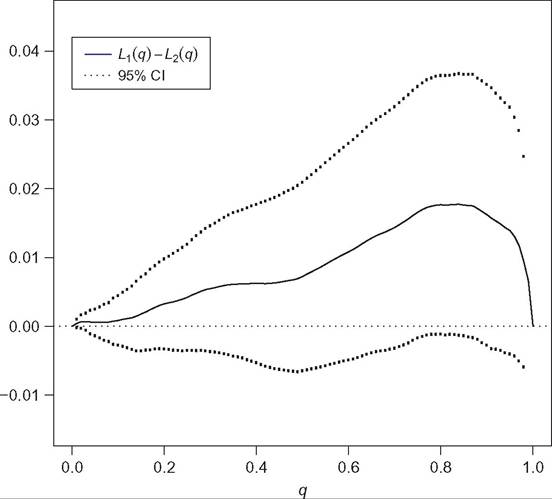
Figure 6.1 Difference between two empirical Lorenz curves, L₁(q)- L₂(q), with 95% confidence intervals. The samples are drawn from the same distribution.

curve ordinate difference is never significantly different from zero; as a result Lorenz dom­inance in the population is not as clear as simple computation from the sample might sug­gest. To be able to make conclusions on dominance or nondominance, we need to test simultaneously that all ordinate differences are statistically greater than zero, or not less than zero. Appropriate test statistics need to be used to make such multiple comparisons.

In this chapter, we will provide a survey of the theory and methods underlying good practice in the statistical analysis of income distribution. We also offer a guide to the tools that are available to the practitioner in this field.

6.1.2 Basic Notation and Terminology

Throughout the chapter, certain concepts are used repeatedly, and so it is convenient to list some of the terms that are used repeatedly.

• Income y. Here “income”; this is merely a convenient shorthand for what in reality may be earnings, wealth, consumption, or something else. We will suppose that y belongs to a set Y = [y,y), an interval on the real line R.

• Population proportion q. For convenience, we will write q E Q :=[0,1].

• Distribution F. This is the cumulative distribution function (CDF) so that, for any y º Y, F(y) denotes the proportion of the population that has income y or less. Where the density is defined, we will write the density at y º Y as f(y). The set of all distri­bution functions will be denoted F.

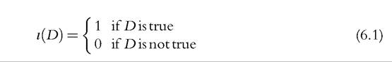
• Indicator function ι(∙). Suppose there is some logical condition D, which may or may not be true. Then ι(∙) is defined as:

6.1.3 A Guide to the Chapter

We begin with a discussion of some ofthe general data issues that researchers should bear in mind (Section 6.2).

6.2.