INCOME POLARIZATION

5.4.1 Discrete Income Polarization

The classic and influential formulation by Esteban and Ray (1994) of an alienation/ identification framework also presents the first axiomatic formalization of polarization.

More formally, it is assumed that the income distribution can be split into a finite number of income classes i = 1,..., n, each with income precisely equal to y_i (another interpretation uses μ_i instead of y_i; see following). Identification felt by individuals is an increasing function I(n_i) of the number n_i of individuals in their income class i. The sense of identification depends only on the number of individuals in a given income cluster. (Extensions of this to account for other characteristics belong to socioeconomic polarization.) The distance of individual i from another individual j is denoted by δ(y_i, yj). An individual with income y_i feels alienation a[δ(y_i, y_j)] toward an individual with income y,∙. The effective antagonism felt by i toward j is represented by a continuous function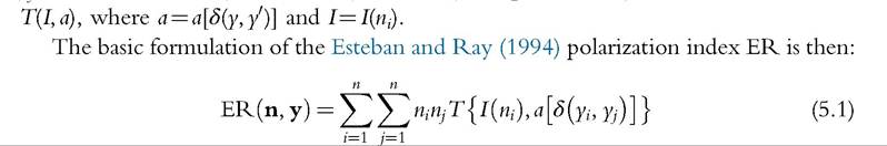

Hence, polarization within a society depends only on the distribution of effective antag­onism,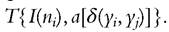Ajustification for the additive formulation of Equation (5.1)

may be provided along the lines suggested by Harsanyi (1953): an impartial observer might want to use the expected value of effective antagonism to judge overall polarization.

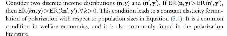
Esteban and Ray (1994) narrow the preceding general formulation by imposing one condition and three axioms on Equation (5.1). The condition is one of invariance with regard to population size: polarization orderings should not change if population sizes are all multiplied by the same number. This is called condition H (for homotheticity).

Condition H

ER’s identification/alienation framework then proceeds with three different axioms. The first two axioms deal with the impact of income movements on polarization. These first two axioms help characterize the structure of the dependence of T(I, a) in Equa­tion (5.1) on alienation. The third axiom considers the impact of changes in the size of population groups; that third axiom defines the sensitivity of antagonism to identification.

Axiom ER 1

Consider a population made of three income groups, as shown in Figure 5.1. Ifthe two smaller and closer groups join together at the average of their incomes, polarization increases.

Axiom ER 1 considers the effect of reducing local alienation on total polarization. The average distance between the two groups originally at x and y and the group at 0 does not change. Average alienation does fall, however, because of incomes x and y moving closer. Axiom ER 1 says that the effect of increased identification of the two groups to the

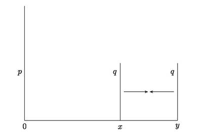
Figure 5.1 Merging two relatively small and close groups at the average of their incomes increases polarization. Note: There are p individuals at income 0, q individuals at income x, and q individuals at income y. The incomes ofthe q + q individuals are changed to (x+y)/2.

right dominates the reduction of alienation. It also implies that the polarization index should be concave in alienation: the effect of the increased alienation between those at incomes 0 and (initial) x dominates the effect of the lower alienation between those at 0 and (initial) y.

Axiom ER 2

Considerapopulation made of three income groups, as shown in Figure 5.2. Ifx moves to the right toward y, polarization increases.

Axiom ER 2 involves two changes in alienation. The first one is a fall in alienation between those at x and those at y. The second is an increase in alienation between those at 0 and those at x. Axiom ER 2 says that the greater proximity of x and y should increase polarization. Axiom ER 2 also implies that the index should be convex in alienation. The combinations of Axioms ER 1 and ER 2 imply that the polarization index should be linear in alienation.

Axiom ER 3

Any new distribution formed by shifting population mass from a central mass of size q equally to two lateral masses each of size p and equally distant away from the central mass increases polarization; see Figure 5.3 for an illustration.

Axiom ER 3 says that absorption (or disappearance) of the middle class into richer and poorer classes should increase polarization. It puts a bound on the relative importance of identification in the measurement of polarization: the effect of the fall in identification felt by middle-class individuals located at x in Figure 5.3 should not be too strong in relation to the effect of the increase in identification felt by those individuals on each side of the middle class.

Esteban and Ray (1994) then show that this framework implies a particular form for Equation (5.1):

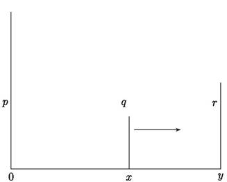
Figure 5.2 Moving x toward y increases polarization. Note: There are p individuals at income 0, q individuals at income x, and r individuals at income y. Incomes x is moved upward.

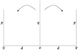
Figure 5.3 Absorption of the middle class into richer and poorer classes increases polarization. Note: There are p individuals at income 0, q individuals at income x, and p individuals at income y = 2x = 2d.

Theorem 4.1

A class of polarization measure satisfies condition H and the three Axioms ER 1, ER 2, and ER 3 if and only if Equation (5.1) has the form:

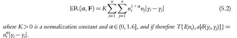
A few remarks may be useful. There are only two degrees of freedom in Equation (5.2), each based on K and α. K is a simple multiplicative constant that has no effect on the ordering of distributions, and α reflects the relative importance of iden­tification and alienation, commonly referred to as a parameter of “polarization aversion.” The polarization measure bears resemblance to the Gini coefficient. Aside from the fact that Equation (5.2) uses the logarithm ofincomes (see following), it would equal the Gini if α were equal to zero. The fact that α can exceed zero distinguishes income polarization and inequality. The larger the value of α, the greater the departure from inequality measurement because of the greater the departure of Equation (5.2) from the pure consideration of income distances.

In the formulation of Esteban and Ray (1994), y_k in Equation (5.2) is taken to be the log of income (or the log of the relevant cardinal variable). One justification is that individuals may be sensitive to percentage differences in income and not to absolute differences in them. Anotherjustification is that the measure in Equation (5.2) is then invariant to proportional changes in all incomes. The use of income logarithms makes, however, the polarization measure to be noncomparable with the Gini index even when the α parameter is set to zero. Furthermore,could be used in such a way as to

make Equation (5.2) invariant to proportional changes and all incomes, when incomes and not income logarithms are used in the formula.

5.4.2 Continuous Income Polarization

The discrete formula in Equation (5.2) provides an index whose application to indicators of welfare that are commonly continuous (such as income) raises difficulties.

Duclos et al. (2004) (DER) address both of these issues in a framework that is rem­iniscent of Esteban and Ray (1994) in surface, but with differences at a deeper level. DER postulates that their polarization index should be proportional to the sum of all effective antagonisms in a continuous distribution,

where f(x) is the (unnormalized) density function—capturing identification—and ∣x — y∣= a is the distance between individuals of income x and y—capturing alienation. The antagonism function T(I, a) is increasing in its second argument, and T(I,0) = T(0, a) = 0.

A functional expression for Equation (5.3) is characterized through the formulation of axioms that, though analogous to those of Esteban and Ray (1994), differ in that the income space is continuous. The domains of the axioms are primarily the union of 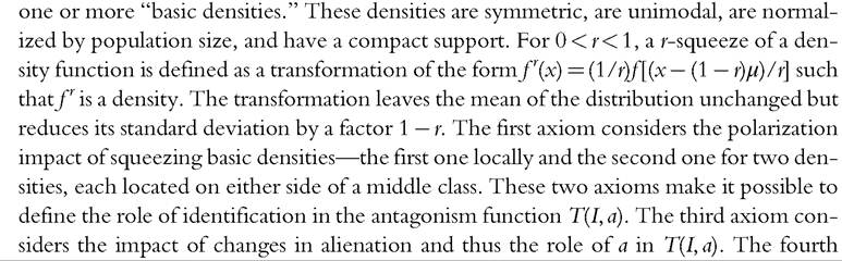axiom is a population invariance axiom.

Axiom DER 1

A squeeze of a distribution made of only one basic density (as shown in Figure 5.4) does not increase polarization.

Alienation diminishes and identification rises following this squeeze; the impact on polarization of greater identification is nevertheless offset by the impact of a decline in alienation. This effectively limits the parameter α (that will be introduced later, see Equa­tion (5.4), and that is the analogue of the α of the discrete formulation ofEquation (5.2)) to be no greater than one because Axiom DER 1 says that polarization should not depart excessively from inequality measurement.

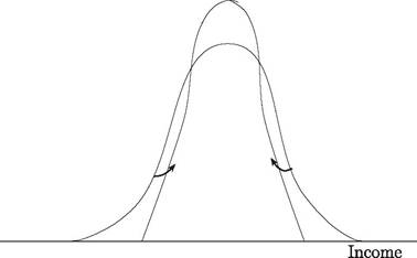
Figure 5.4 A squeeze of a basic density does not increase polarization.

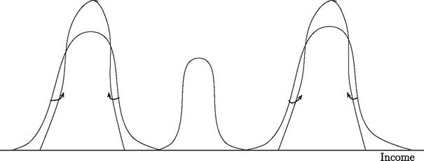
Figure 5.5 A double squeeze cannot reduce polarization.

Axiom DER 2

Ifthe distribution of a symmetric density has three poles (see Figure 5.5), then a squeeze of the outer poles does not decrease polarization.

The decline of intergroup alienation in the outer poles is counterbalanced by the rise ofidentification. Axiom DER 2 is the “defining” axiom of polarization: It differentiates polarization from inequality. It also puts a lower bound on the parameter α in Equa­tion (5.4): It should not lie below 0.25 for the fall in local alienation (the alienation within each extreme group) to be outweighed by the increase in identification. The axiom also implies that the polarization index should be concave in alienation—for the fall in larger alienation values (the more extreme distances from the middle fall following the squeeze) not to have too large an impact on total polarization.

Axiom DER 3

Ifa symmetric density has four poles and if each of the two middle poles shifts to the nearer outer pole, as in Figure 5.6, then polarization must go up.

Figure 5.6 shows a fall in local alienation combined with an increase in larger alien­ation values (an increase in the larger distances between groups). This implies that polar­ization should be weakly convex is alienation; the effect of a fall in smaller distances should be outweighed by a similarly sized increase in the value of larger distances. Axioms DER 2 and DER 3 imply that polarization should be linear in alienation.

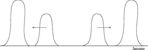
Figure 5.6 A symmetric outward slide must raise polarization.

Axiom DER 4

If the polarization index for one distribution is higher than for another one, then it remains higher when both populations are identically scaled.

This axiom states that polarization orderings should be invariant to population size. It plays a role similar to Condition H given earlier for discrete income polarization. It links identification and polarization through a constant elasticity function in Equation (5.4). DER then shows that:

Theorem 4.2

The index Equation (5.3) satisfies Axioms DER 1, DER 2, DER 3, and DER 4 if and only if it is proportional to:

Making polarization invariant to proportional changes in all incomes can be done by multiplying DER(α) byFor α = 0, the measure would be equivalent to the Gini coef­

ficient. Note, however, that Theorem 4.2 excludes the Gini index: the Gini index would indeed fall following the squeeze of Figure 5.4, which would violate Axiom DER 2.

The DER(α) polarization index can be decomposed into identification and alienation components. For a particular value of α, average à-identification can be expressed as

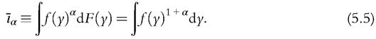
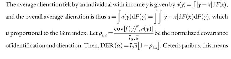
that greater multimodality in the density is likely to translate into greater ι_α and into greater polarization—this effect becoming stronger when α is larger. Greater inequality and thus greater average alienation a will also mean greater polarization. Finally, a greater covariance ρ_ia between identification and alienation will raise polarization.

5.4.3 Discrete Income Polarization with Endogenous Grouping

The DER(α) index effectively sets the number of possible income groups to infinity. Each group displays perfect internal homogeneity, being associated with one and only one income level. That removes the need for selecting either the number or the position of income groups.

We might, however, think of measuring income polarization on the basis of a finite and prespecified number of income groups and select their position to maximize internal group homogeneity. Choosingpositions to maximize internal homogeneity has the advantage of maximizing local identification and minimizing local alienation—but because individuals in a given group do not all have the same income with discrete income groupings, there will necessarily remain internal heterogeneity, even after such an optimization procedure.

Such an approach is used by Esteban et al. (2007) on the Esteban and Ray (1994) index, using a continuous variable such as income and specifying the number of income groups to be used but not their precise location. Clustering into a finite number of classes introduces errors in the measurement of continuous income polarization. This clustering introduces an approximation error ε(F). The greater the error, the greater the level of internal heterogeneity, the lower the level of internal identification, the greater the level of local alienation, and the greater the likelihood of a bias in using ER(α, F) as an index of continuous income polarization. An “extended” polarization index that attempts to cor­rect for such biases is given by:

where α is the usual polarization sensitivity parameter and σ is a parameter that weights the measurement error. The approximation error is specified as

and the problem is set to minimize ε(F) for a given number n of groups. From Equa­tion (5.7), it can be seen that it is equivalent to minimizing the sum of the within-group Gini indices or, alternatively, to minimizing the sum of within-group alienation. The solution is denoted by F*, with

where GB(.) is between-group Gini coefficient of F*. The Esteban et al. (2007) index is then

Note thatis originally meant to capture the effect of one error, the over­estimation byof income identification in a context in which incomes are

artificially grouped. Another error also exists, however, and comes from the under­estimation byof income alienation in a context in which local alienation

is removed through a discrete formation of income groups. The true approximation error of the Esteban and Ray (1994) is therefore quite complicated and should attempt in particular to account both for the identification and the alienation errors of group­ing individuals. The formulation of the error should also be consistent with the special form taken by the Esteban and Ray (1994) index; Equation (5.9) takes the awkward shape of a difference between noncomparable functions whenever α is different from zero.

An example of a difficulty created by the form of Equation (5.9) is noted in Lasso de la Vega and Urrutia (2006); the Esteban et al. (2007) measure may fall when groups move farther away from each other because identification errors may increase when this hap­pens, with a resulting fall in Equation (5.9). The alternative index proposed in Lasso de la Vega and Urrutia (2006) is given by

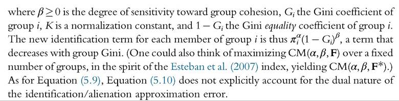
5.5.