BIPOLARIZATION

5.5.1 Measures of the Size of the Middle Class

Income polarization captures the existence and the importance of an arbitrary number of income poles; bipolarization measures the extent to which a population is divided into two separate groups.

between groups. Measures of the middle class have, however, relied on definitions that have often been imprecise and heterogeneous.^[176]

The size (and the composition) of the middle class is important for a number of eco­nomic and social aspects of development. The middle class is a key provider of skilled labor and constitutes an important market for domestic goods and services. The middle class also directly or indirectly provides a large part of a country’s tax revenue. A higher share of income for the middle class has been empirically associated with higher incomes and higher growth (Easterly, 2001) as well as with more education, better health care, better infrastructure, better economic policies, less political instability, less civil war and ethnic tension, more social modernization, and more democracy. One reason fre­quently suggested for this is that a larger-sized middle class is associated with societies with lesser poles at each extreme of the income distribution, thus facilitating political and social harmony and more stable and stronger economic development.

As in the inequality literature, much of the analytical efforts have centered around the construction of indices.

The most influential initial measures of the size of the middle class have then relied on the position of two income cutoff points around the median and on defining the middle class as the share of the population with income within these cutoff points. The middle class is hence defined as the share of the population with incomes between 75% and 125% of the median income by Thurow (1984); Blackburn and Bloom (1995) broaden that middle income range to 60—225% of median income; in Leckie (1988), the middle class is defined on the basis of an income range of 85—115% of median wage. The resulting middle-class indices, denoted as M, is then the share of the population found within these cutoff points. This approach is illustrated graphically using either the density function of the income distribution (Figure 5.7) or the cdf F (Figure 5.8). If the density function is used, the index Mis the area situated under its curve and between the lower and the upper bounds of the income range. With the cumulative distributive function, the index M is the vertical distance between the values of the cdf evaluated at the two cutoff points.

A people space can also be used. Levy (1987) considers the income share of the middle three-fifths of the population as the size of the middle class.

Levy’s (1987) index was criticized by Foster and Wolfson (2010/1992) for measuring something other than the size of the middle class or bipolarization. Foster and Wolfson (2010/1992) argued that the index can be considered to be a sound measure of the skew­ness of the distribution; it should not be viewed, however, as a good index of the size of

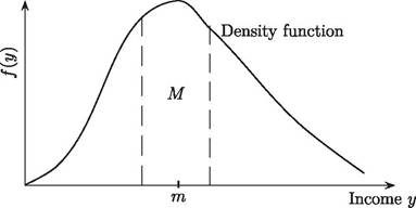
Figure 5.7 Finding the size M of the middle class with a density function.

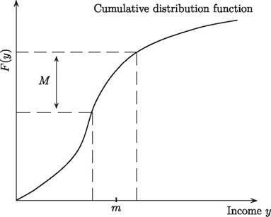
Figure 5.8 Finding the size M of the middle class with a cumulative distribution function.

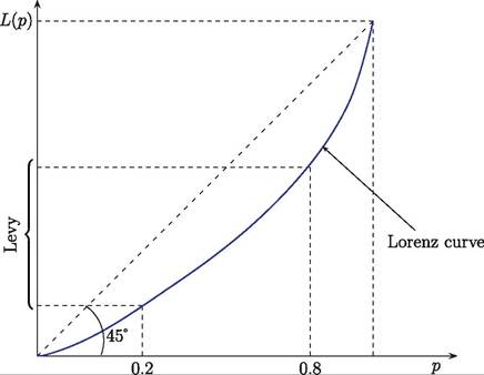
Figure 5.9 Lorenz curve and the Levy (1987) index of the size of the middle class.

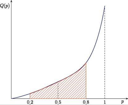
Figure 5.10 Quantile function.

the middle class or of the extent of bipolarization because it fails to measure “spreads” on each side of the middle class. One way to see the problem is to observe that any symmetric distribution will exhibit exactly the same value for the Levy index. For any symmetric distribution, we have indeed that L(1 — p) — L(p) = 1 — 2p for all p. For the specific case of p = 0.2, the index yields a value of 0.6, which is therefore the value of the Levy index for all symmetric distributions, however far incomes may be from the median and how­ever bipolarized these incomes may be.

The fact that Levy-type measures fail to capture spreads on each side of the median can be illustrated in several fashions. For instance, an increase in any quantile

Q(p) for p 2 [0.5,0.8] will increase the Levy measure of the size of the middle class (because L(0.8) will increase and L(0.2) will fall); that, however, will increase the spreads from the median and should therefore conceivably increase bipolarization. Similarly, a fall in Q(0.1) will decrease L(0.2) and increase the Levy measure of the size of the middle class, although that should arguably lead to an increase in the level of bipolarization. Increases in bipolarity that occur entirely within p 2 [0.2,0.8] will not change the Levy measure, although they should reasonably impact bipolarization.

5.5.2 Two Basic Properties of Bipolarization Indices

From the preceding, it is clear that quantifying levels of bipolarization and of the size of the middle class may be treacherous conceptually and thus methodologically. To solve part of the ambiguity, it may be useful to agree on basic properties that the methodolog­ical exercise should obey. The two basic properties of bipolarization measurement on which most of the bipolarization literature has insisted are the effects of “increased spread” and “increased bipolarity” (or increased bimodality in Wolfson, 1997).⁸

Consider a discrete population of two income groups, B and D, distributed around median income C and as drawn in Figure 5.11. Now assume that those below and above the median line move away from it; that is, the poorer (at B) become poorer until their income becomes A, and the richer (at D) become richer until their income is at E. Each of these movements away from the middle is called an “increased spread.” When this occurs, polarization and inequality are said both to increase. The new distribution is indeed obtained from the old one by a mean preserving regressive transfer across the mid­dle; this increases distances between individuals (and therefore increases inequality), and it

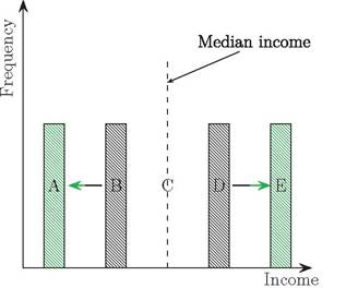
Figure 5.11 Increased spread.

A recent survey of the bipolarization literature can be found in Nissanov et al. (2010).

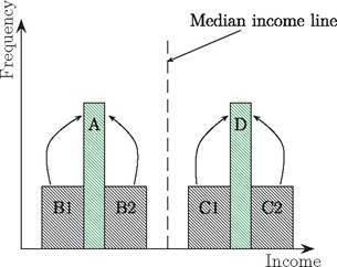
Figure 5.12 Increased bipolarity.

also increases all distances from the middle (and thus raises bipolarization). As in the inequality literature, these movements can be thought to be ethically regrettable.

Figure 5.12 illustrates the property of increased bipolarity. Increased bipolarity is the result of two “spread changes,” an “increased spread” and a “decreased spread.” Suppose that, below the median, populations with income B1 and B2 cluster at their mean income A and, above the median, populations with income C1 and C2 cluster at their mean income D. Inequality decreases, but polarization can be reasonably said to increase. With increased bipolarity, the average positions of the masses on each side of the median do not change, and the median themselves are not altered, but the distributions on each side of the median are tightened up. During the movement, individuals nearer to the middle move away from it, whereas individuals farther from the median move toward it. The move­ments of the first group increase the spreads from the median, whereas the movements of the second group of individuals reduce those spreads. Overall, bipolarization increases because the first movements are thought to carry more weight than the second ones.

Increased bipolarity thus distinguishes fundamentally polarization from inequality. Any progressive transfer leads to an unambiguous decrease in inequality, irrespective of the location of the transfer. Bipolarization also falls when the transfer takes place across the middle. Bipolarization is said to increase when the transfer occurs on one side of the middle.^[178] A concern about polarization can thus lead us to reject a transfer that would otherwise reduce inequality, where that transfer would take people away from the median.

Much of the literature on bipolarization takes these two properties as given and then proceeds into alternative directions. The first direction leads to the construction of bipo­larization indices that are consistent with these two properties. These indices provide com­plete bipolarization orderings of distributions. The second direction provides dominance curves for making partial bipolarization orderings. The design of these curves draws from the well-known applications of stochastic dominance in the inequality literature.

It is also on this basis that Foster and Wolfson (2010/1992) (FW) set their influential paper. (The paper was published in 2010 in the Journal of Economic Inequality as a “rediscovered classic,” having circulated until then as a 1992 working paper.) FW intro­duce two bipolarization curves as well as a new Gini-like index of bipolarization. The first curve says that bipolarization is greater when the size of the middle class is smaller, viz., when the distances to the median are larger. The second bipolarization curve says that bipolarization is higher when the average distance from the median, on either side of the median, are larger.

The index proposed by FW equals twice the area between the Lorenz curve and the tangent to the Lorenz curve at median income (this area being multiplied by μ). The index can also be expressed as a function of within- and between-group inequalities: the larger the extent of between-group inequality, the larger is bipolarization, and the larger the level of within-group inequality, the lower is the level of bipolarization. We now examine this in more details.

An income distance between two quantiles at percentiles q and q⁺ is defined by 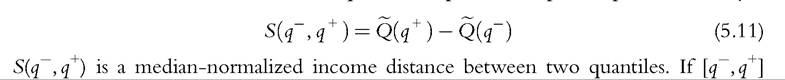overlaps 0.5, it can also be thought of as a measure of the size of the middle class. When S is large, there are fewer individuals near the middle, and consequently the middle class is deemed smaller and there is more bipolarization. FW (see also Wolfson, 1994) define a first-order polarization curve as:

for 0 ≤p ≤ 1. For each p, S(p) is the distance that separates median income from the income of the person situated at the pth percentile. This is illustrated in Figure 5.13. Two distances from the median are shown in the upper panel,The bot­

tom panel of Figure 5.13 mirrors the left-hand side of the upper panel. It draws a first- order bipolarization dominance curve “looking a bit like a lopsided gull” (Wolfson, 1994, p. 355).

FW also define a second-order polarization curve as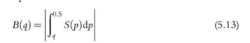

for 0 ≤ q ≤ 1. B(q) is the area under the S(p) curve between points q and 0.5. This is also shown in Figure 5.13 as hatched areas representing B(q~) and B(q⁺). Figure 5.14 shows the shape of a typical B( p) curve, and how its side values B(0) and B(1) can be expressed as functions of the Lorenz point L(0.5). An important point is that B(q) is obtained by inte­grating “inward” to the median (p from q to 0.5); the usual stochastic dominance curves integrate from 0.

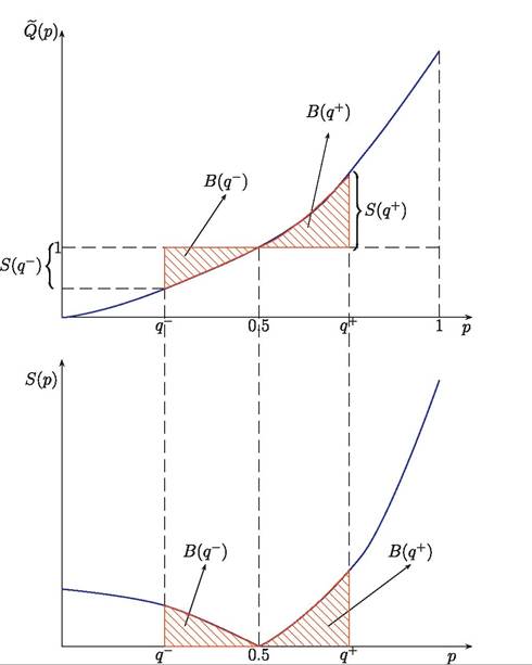
Figure 5.13 First-order bipolarization curves.

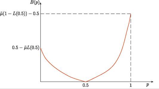
Figure 5.14 Second-order bipolarization curve.

5.5.3 Bipolarization Dominance

The curvesjust introduced can be used for descriptive as well as for normative purposes. They are called dual curves because they are a function of percentiles p. Analogous dual curves in welfare economics include quantile, Lorenz, generalized Lorenz, poverty gap, and cumulative poverty gap curves—see, for instance, Duclos and Araar (2006) for def­initions and a discussion. Primal curves also exist. These primal curves are a function of income levels. These incomes need to be expressed as proportions of the middle (the median, usually) for bipolarization comparisons. A natural first-order primal curve for such comparisons is given by F(λm) — 0.5 for λ > 1, namely, the proportion of the pop­ulation found between the median itself and λ times the median, or the expression 0.5 — F(λm) for λ > 1, that is, the proportion of the population found between λ times the median and the median. Both of these measures are popular features of the measure­ment of the size of the middle class—seefor instance Morris et al. (1994). They are illus­trated in Figure 5.15 (recall that.

Increases in spreads from the median will decrease each of these two expressions, F(λm) — 0.5 and 0.5 — F(λm). Increases in bipolarity will increase these expressions at some values of λ and will reduce them at other values of λ.

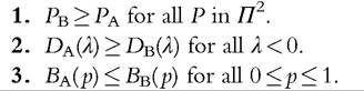
Let Π¹ then be a class of bipolarization indices P that are functionals of F, population size invariant, monotonically increasing in Q(p) forp > 0.5 and monotonically decreasing in) for p< 0.5. The following conditions can then be shown to be equivalent:

5.5.3.1 First-Order Bipolarization Dominance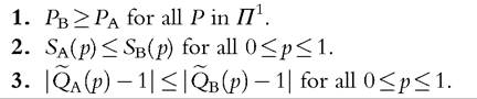

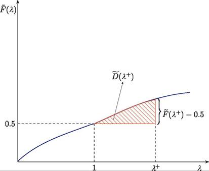
Figure 5.15 Average distance from bipolar extremes.

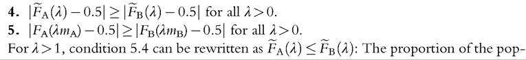
ulation with income less than λ times median income (a frequently used relative poverty line) should be lower in A for A to be less bipolarized.

These results can be extended to the case of symmetry of bipolarization indices with respect to distances on each side ofthe median. Let Π^S1 be a class of bipolarization indices P that are functionals of F (y), are population invariant, and are monotonically increasing

5.5.3.2 First-Order Symmetric Bipolarization Dominance

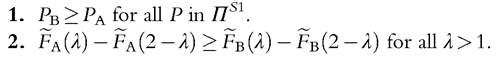
This is equivalent to comparing the shares of the population within a distance λ — 1 of the median (Duclos and Echevin, 2005), which is also a frequently used and simple descrip­tive statistic of the size of the middle class.

The welfare economics literature often stresses the view that some income levels in the income distribution are more important than others, in the sense that changes in these incomes engender greater changes in social evaluation functions (such as social welfare functions or inequality indices). The same view is put forth in the bipolarization literature through the application of the increased bipolarity property, which technically says that indices of bipolarization should be concave in distances from the median and conceptu­ally means that increases in smaller spreads from the median have a greater impact on bipolarization than rises in larger spreads. The curves that are used to establish dominance on the basis of these indices cumulate income distances from the median, in the manner of B(p) for dual curves and in the manner of

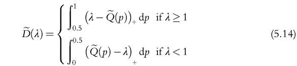
for primal curves. Figure 5.15 illustrates D(λ) for λ⁺. It can be seen as the integral of the F(λm) — 0.5 (for λ > 1) and 0.5 — F(λm) (for λ < 1). From Equation (5.14), it can also be seen that D(λ) can be expressed as the sum of the distances between median-normalized incomes Q and a threshold λ. This is analogous to the aggregation of poverty gaps in the poverty literature: the larger the sum of poverty gaps, the greater is poverty; the larger the sum of the gaps between normalized incomes and a threshold on each side of the median, the greater is bipolarization. D(λ) can also be understood as the average distance from bipolar extremes (λ) on either side of the median.

Let ∏² be a class of bipolarization indices P that are functionals of F, population invariant, monotonically increasing in Q(p) for p > 0.5, monotonically decreasing in Q(p) for p < 0.5, and concave in Q(p). The following conditions are then equivalent.

5.5.3.3 Second-Order Bipolarization Dominance

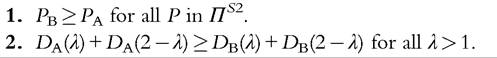
As discussed earlier, this can be extended to the case of symmetric of bipolarization indi­ces with respect to distances on each side of the median. Let Π^s2 be a class of bipolari­zation indices P that are functionals of F, population invariant, and monotonically increasing and concave in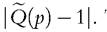The following conditions are then equivalent.

5.5.3.4 Second-Order Symmetric Bipolarization Dominance

A natural question is whether these bipolarization partial orderings have power empir­ically, namely, whether it is possible to rank bipolarization across distributions using them. The comparisons of 29 Luxembourg Income Study (LIS) countries found in Duclos and Echevin (2005) show some evidence of this. The comparisons are made with and without statistical testing of the differences between the curves; it is more difficult to distinguish the curves statistically than numerically. ⁰ Symmetric and asymmetric bipo­larization dominance tests are also performed; symmetric tests have naturally more power. Overall, Duclos and Echevin (2005) found that first-order dominance is found statistically across 32% of the 406 possible pairwise comparisons; that percentage increases to 55% for symmetric first-order dominance testing and to 73% for second-order sym­metric dominance.

5.5.4 Bipolarization Indices

Specific numerical indices are frequently used to summarize and compare income distri­butions and have the advantage of providing complete orderings over distributions. FW propose one such index with two principles in mind:

1. The index should conform to basic underlying notions of the concept being mea­sured; for example, inequality measures should be Lorenz-consistent, the Lorenz curve being the gold standard in comparing inequality robustly and graphically. In the case of bipolarization, FW base their index on the second-order dual bipolariza­tion curve B(p), which is the bipolarization analogue of the Lorenz curve.

10

See Chapter 6 of this Handbook for a coverage of some of the estimation and inference issues involved in comparing distributions.

2. The index should be easily understandable. For example, the Gini coefficient can be expressed as twice the area between the Lorenz curve and the diagonal of equality.

FW follow a similar procedure in proposing their index.

The bipolarization index of Foster and Wolfson (2010/1992) is then defined as

⁾ which is twice the area beneath the second-order bipolarization curve B( p). FW is there­fore necessarily consistent with a partial ordering based on comparing B(q). It is also sim­ple to understand.

FW also has quite a few other interesting features. It is, for instance, linked to the Gini index and the line tangent to the Lorenz curve at the median income. Let the average distance between incomes under the median and incomes above the median be given by: 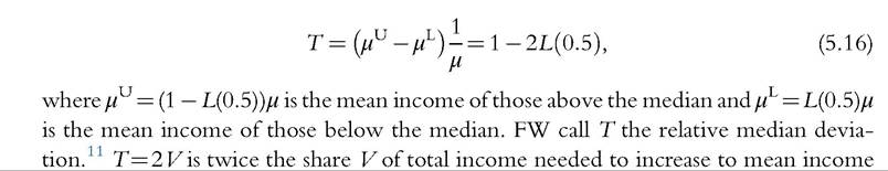the incomes of those below the median. Thus, it can be measured as twice the vertical distance from the first diagonal to the Lorenz curve at the level at which the cumulative percentage of the population equals 0.5. This is shown in Figure 5.17.

Another expression for T is given by integrating S(p):

so that T is twice the area under the first-order polarization curve normalized by μ—see Figure 5.13.

T is also twice the area of the quadrilateral 0ABC in Figure 5.17. This has two con­sequences: first, Tis greater than the Gini coefficient G and, second, the area between the Lorenz curve and the tangent line (the light gray area in Figure 5.17) is never zero when G is nonzero.

Foster and Wolfson (2010/1992) then show that

The index FW is a scaling up (by the skewness measure (μ/m)) of the light gray area of Figure 5.17. It is thus simple to construct from such basic statistics as mean income, median income, the Gini coefficient, and the relative median deviation.

¹¹ This is different from the relative mean deviation, which is given by 2(F(μ) — L(F(μ))).

Figure 5.16 Maximum bipolarization.

When a distribution is perfectly bimodal, half of the population has zero income and the other half has income equal to 2μ. This case of perfect bimodality is shown in Figure 5.16. Maximal FW bipolarization is given by twice the area covered by the tri­angles that lie between the Lorenz curve of the bimodal distribution and the 45° line that touches the horizontal axis atp = 0.5. Each triangle has an area of 0.125, as shown on the figure. Twice those areas equals 0.5, which is the maximum value attained by FW. FW equals zero in the case of a perfectly equal distribution. Wolfson (1994, 1997) prefer to redefine FW by multiplying it by 2, so that the new index ranges from 0 to 1.

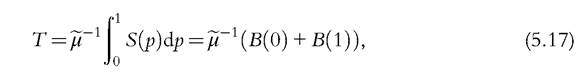
The polarization index FW can also be expressed as a function of components of the Gini coefficient, between-group inequality, and within-group inequality. Divide the population into two groups, one made of individuals with income below the median and the other one made of individuals with income above the median. Give income μ^b to individuals below the median and μ^U to individuals above the median. GB(F) is the between-group Gini coefficient of this new income distribution, which has no within-group inequality. The difference GW(F) = G(F) — GB(F) is a measure of within-group inequality and is a population-weighted sum of Ginis within the two groups.

An illustration of this decomposition is given in Figure 5.17. The three values of the Lorenz curve at points 0, 0.5, and 1 are joined to form a between-group Lorenz curve, a

Figure 5.17 Polarization, relative median deviation, and within- and between-group inequality.

piece-wise linear curve. GW(F) is twice the area between the original Lorenz curve and the newly graphed between-group Lorenz curve; GB(F) is twice the area captured by the between-group Lorenz curve, that is, the area between it and the 45° line. The area of the triangle formed by the between-group Lorenz curve and the diagonal equals [0.5 — L(0.5)]/2, such that between-group inequality equals GB(F) = 0.5 — L(0.5) and that T = 2GB(F) is twice the between-group inequality term. Given this, an alternative expression for the FW index is therefore

Equation (5.19) is a function ofbetween-group inequality minus within-group inequal­ity as measured by the Gini index and with the two groups, respectively, above and below the median. This nicely shows how the bipolarization index FW is influenced both by spreads from the median and by bipolarity. Increases in spreads from the middle raise GW; increases in bipolarity reduce GW. Both effects increase bipolarization. Changes in spreads from the middle have a larger impact on bipolarization when the spreads are initially small: increases in spreads from the middle raise between-group inequality, but within-group inequality indeed falls faster when those closer to the median move away from it.

We use 2004 Canadian data from the LIS to illustrate some of these expressions. The estimates of the Gini for those below and above the median are G_l = 0.206 and G_u = 0.213, respectively; the data also yield estimates ofand L(0.5) =

0.286. This leads to T = 0.430, namely, the relative median deviation and twice the share of total income needed to increase to mean income of those below the median. The between-group Gini index (GB = 0.5 — L(0.5)) is found to be 0.215, and the

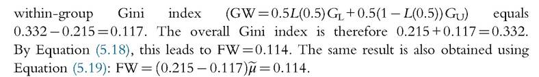
As shown in Equation (5.19), inequality and polarization rise together when inequal­ity between the two groups rises; they move in opposite directions when within-group inequality declines. When between-group inequality increases, inequality and polariza­tion rise simultaneously—this corresponds to a greater spread; when within-group inequality (GW(F)) decreases, inequality decreases too, but polarization rises, corre­sponding to increased bipolarity.

5.5.5 Income Polarization and Bipolarization

Note that increased bipolarity leads to lower inequality on each side of the median, but not necessarily to poles that are necessarily more defined on each of these sides. Consider, for instance, Figure 5.18. The initial distribution (shown by the 45°-hatched rectangles) has four equally sized separate groups, two on each side of the median. Say that the two groups on the right-hand side each split into two smaller groups (leading to the 6 — 45° - hatched rectangles, two on the left-hand side and four on the right-hand side) following an increase in bipolarity on the right-hand side of the distribution. Within-group inequality has increased, and between-group inequality has been left unchanged. Bipo­larization should therefore be judged to have increased, but is this also the case for polar­ization? It may instead be argued that the poles of the distribution have now become less well defined and that income polarization has fallen.

This important distinction between income polarization and bipolarization can be pushed further. It should be clear that concepts and measurement of income polarization and bipolarization are related and yet different. Conceptually, income polarization is con­cerned with the existence of multiple groups; bipolarization deals with the existence of

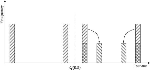
Figure 5.18 Does increasing bipolarity increase polarization?

two bipolar groups. From a measurement perspective, different functional restrictions are also imposed. Income polarization is based on the average antagonism generated by the mixture of identification and alienation. Bipolarization is a function of distances from a middle. It is therefore not surprising that income polarization and bipolarization order­ings may clash.

Axiomatically, there are also similarities and differences across the two frameworks. For instance, the properties of bipolarization measurement imply some of the commonly used income polarization axioms. The property of increased spread implies Axioms DER 1 and DER 3; the property of increased bipolarity implies Axiom DER 2. Thus, bipolarization indices such as FW obey Axioms DER 1, DER 2, and DER 3 (and DER 4 as well because of population size invariance). But the converse is not true. The DER axioms do not imply the two fundamental properties of bipolarization measurement. This also suggests that (leaving aside the differences in the initial functional restrictions, see Esteban and Ray, 2012) the income polarization framework is more flexible than the bipolarization one, as intuition also suggests because the income polarization framework is set over an arbitrary number of groupings.

Because of this greater flexibility, the DER indices can fail, however, to obey the increased spread and the increased bipolarity properties (again, see Esteban and Ray, 2012). This is because the movements involved in these properties can decrease identi­fication sufficiently to lead to a fall in average antagonism and thus in income polarization. Again, a demonstration of this is shown in Figure 5.18, where the movements increase bipolarization but may decrease income polarization.

Conversely, bipolarization indices such as FW can fall following squeezes of local dis­tances that increase local identification. For instance, a squeeze of each of three equally sized and equally spaced symmetric basic densities will always decrease FW, but will also always increase DER. (This is in fact true for squeezes of any odd number of such sym­metric groups.) Again, the source of the clash comes from the conceptual distinction between distances across well-identified groups and distances of those groups from a middle.

5.5.6 Extensions

Various extensions of the FW index have been proposed. Most of them rely on intuitive alternative applications of the spread/bipolarity framework. One fruitful general approach is to think of distances from the median as the variable of normative interest and to use well- known aggregation techniques from welfare economics to aggregate these distances in a manner that ensures that desirable properties are fulfilled. Note that, for the measurement of polarization, those properties then apply to distances from the median: in welfare eco­nomics, the same properties normally apply to distances from the mean or from other incomes—see, for instance, Chapter 4 in Duclos and Araar (2006).

Wang and Tsui (2000) proposed two types of extensions, both of which are axiom- atically characterized. In both cases, income distances from the median are aggregated. The first type of aggregation uses rank weighting to aggregate the distances in a manner analogous to Donaldson and Weymark (1980) and Yitzhaki (1983). The measure is defined as

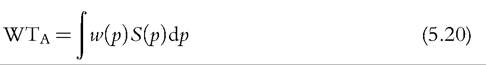
where w(p) is positive and increasing for p ≤ 0.5 and positive and decreasing for p > 0.5. Positivity of p is needed for the increasing spread property to hold: Any increase in S(p) must raise WTA. Increasingness of w(p) for p ≤ 0.5 and decreasingness of w(p) forp ≥ 0.5 are needed for the increasing bipolarity property to hold as well. Makdissi and Mussard (2010) used classes of such indices to assess the impact of tax reforms.

Wang and Tsui (2000) also considered polarization measures defined as transformation of distances from the median and normalized in such a way that there is no polarization when income is equally distributed across all individuals. A class of such indices is given by

where ψ(u) is a continuous function. The class of polarization indices WT_b satisfies the axioms of increasing spread and of bipolarity if and only if ψ(u) is strictly increasing, strictly concave, and with ψ(0) = 0. A constant elasticity formulation for ψ emerges if rankings of nonnormalized distances must always be the same as those for normalized distances from the median. This yields the polarization class of indices

where r 2 (0,1). The larger the value of r, the more sensitive are the polarization indices to the deviations of richer persons’ incomes from the median.

Inspiration from the inequality literature can also be used to generalize the aggrega­tion of distances from the median that Foster and Wolfson (2010/1992) and much of the subsequent bipolarization literature have adopted. An example of this is Chakravarty and Majumder (2001)'s exploration of the use of the Atkinson (1970), Kolm (1969), and Sen (1973) inequality indices for the measurement of bipolarization—see also Chakravarty (2009, section 4.3). By constructing, inter alia, “equally distributed equivalent incomes” on the separate distributions of incomes lower and greater than the median, it is possible to take into account inequality on each side of the median to assess by how far the two groups are from the middle of the entire distribution. When the welfare evaluation func­tion is of the Gini type, such procedures simplify to the Foster and Wolfson (2010/1992) measure of bipolarization.

Rodrlguez and Salas (2003) follow in FW’s footpath by applying a sensitivity param­eter to weight the subgroup decomposition of the Gini coefficient into between and within-group inequality. Using the Donaldson and Weymark (1980) and Yitzhaki (1983) single parameter/extended Gini coefficients, they propose a bipolarization index of the form

where ν is an inequality aversion parameter—see Duclos and Araar (2006) for a discus­sion. Aprogressive median-preserving transfer within (between) the two groups on each side of the median increases (reduces) polarization.

5.5.7 Absolute and Relative Bipolarization Indices

The literature on inequality offers both absolute and relative inequality indices. Absolute inequality indices are invariant to translations of every income by the same constant. Rel­ative inequality indices are invariant to changes in the scaling of all incomes; they are homogeneous of degree zero in all incomes.

Similar distinctions can be (and have been) made in the bipolarization literature. Chakravarty et al. (2007) discuss how the second-order bipolarization curve of Foster and Wolfson (2010/1992) can be made absolute, in the sense of being invariant to trans­lations of every income by the same amount. Integrating the area under this absolute curve leads to an absolute version of the relative bipolarization index of Foster and Wolfson (2010/1992). The absolute inequality indices of the Kolm (1969) and Donaldson and Weymark (1980) types can also be used to weight the sums of absolute distances from the median.

Chakravarty and D’Ambrosio (2010) furthered these distinctions by defining interme­diate bipolarization indices, namely, bipolarization indices that generate as special cases absolute and relative bipolarization indices. More precisely, we may want a distribution of income y and a distribution y + c[γy +(1 — γ)] to exhibit the same level ofbipolarization, where c > 0 is a scalar. This implies that it is the distances S(p) m∕(γm + (1 — γ)) that must be aggregated in the measurement ofbipolarization. The bipolarization curves of Equa­tions (5.12) and (5.13) then become intermediate polarization curves and are given by

When γ = 0, an absolute polarization curve is obtained; γ = 1 yields a relative polarization curve. These curves can be used to derive an intermediate polarization index analogous to

that of Foster and Wolfson (2010/1992), given by the area below the intermediate bipo­larization curve. This yields:

The intermediate polarization index IFW becomes an absolute index if γ = 0 and a rel­ative one if γ = 1.

We may also wish distributional rankings to remain invariant to the choice of mea­surement units. This invariance property (known as unit consistency) does not require indices to be invariant to changes in monetary units (such as cents or dollars); it only requires the distributional orderings not to be affected by such changes. The implications of such a property for the measurement of bipolarization are explored in Lasso de la Vega et al. (2010), following Zheng (2007) for the measurement of inequality. The results make use of Krtscha-type (Krstcha, 1994) intermediate polarization indices, indices that rank polarization identically across distributions A and B if and only if

γ 2 [0,1] can be regarded as a degree of bipolarization intermediateness. The extreme values of γ equal to 0 and 1 correspond to absolute and relative polarization measures and orderings. Krtscha-type bipolarization orderings can then be made on the basis of m(^lz'ⁱS(p). Lasso de la Vega et al. (2010) show that the only type ofbipolarization order­ings that are unit consistent are those of the Krtscha type.

5.5.8 Bipolarization with Ordinal Data

It is not difficult to think of applications of bipolarization to contexts in which the welfare variable is discrete and ordinal. Examples of such variables include education, class, and positional statuses as well as health indicators. Although such indicators have ordinal con­tent (values of the variables can be ranked), the fact that they are not cardinal makes it difficult to mean or median normalize them, as is typically done for inequality analysis.

It may, however, still be possible to compare the extent ofbipolarization over distri­butions of such variables. An example of such an exercise is found in Apouey (2007) for distributions of discrete and ordinal self-assessed health (SAH) data.^[179] It is first assumed that a distribution exhibits no bipolarization when everybody has the same health con­dition, and that a distribution exhibits maximal polarization if half the population has the lowest SAH indicator and the other half has the highest one. It is then assumed that bipolarization can be expressed as the sum of the distances ∣F(i) — 0.5∣ for each level of category i, i = 1,..., n, ranked from lowest to highest values.

12

It is then shown that

where K is a strictly positive constant and η > 0 is the weight on the median category, which is the only bipolarization measure that satisfies a population invariance axiom and an increasing spread axiom. Bipolarization is maximal when F(i) = 0.5 for all i < n. An axiom of increased bipolarity is obeyed if and only if η∈]0, 1[ and therefore if Apo(η, F) is convex in F(i).

Movements of F(i) away from 0.5 increase bipolarization more if F(i) is initially close to 0.5. An increase in bipolarity moves values of F(i) close to 0.5 away from it and moves more extreme values of F(i) closer to 0.5. Such an increase in bipolarity thus increases bipolarization.

5.6.