APPLICATIONS
Although our discussion so far has remained at an abstract level, the different positions described suggest different approaches to many applied issues that are of great importance for measuring inequality.
An important application is the booming literature on socioeconomic inequality and racial disparities in health, in which the issue of cumulative deprivation (with respect to income and health) plays a crucial role. Because this literature has been discussed in great detail in Fleurbaey and Schokkaert (2012), we will not repeat this analysis here. We will illustrate the practical relevance of the previous sections by focusing on three applications. We first discuss the issue of household equivalence scales and (related to that) the measurement of intrahousehold inequality. We will then look at the different methods that have been proposed to include the value of public goods and services into the analysis of inequality. Our third application is the analysis of world inequalities, including a discussion of purchasing-power parity (PPP) indices. In each of these subsections, we do not go into the technical details but focus on the relationship with the normative analysis in the previous sections.2.5.1 Household Equivalence Scales
It is widely agreed that the quality of social relations is one of the most important dimensions of life. For many people this is particularly true for their relationship with a partner and the quality of their family life. Also the presence of children changes life deeply (for better or for worse). Therefore, it seems natural to include these family-related dimensions in a broader view of well-being. Family relations have been introduced in the capability approach, often with a focus on gender issues (see, for instance, Nussbaum, 2000; Robeyns, 2003). Moreover, family relations have been shown to have a strong effect on happiness or life satisfaction.
A famous example is offered by Blanchflower and Oswald (2004). The authors estimate that a lasting marriage (compared to widowhood as a natural experiment) is worth $100,000 a year. As far as we know, there are no applications in the equivalent income tradition yet.[79] It would not be difficult to derive equivalent incomes on the basis of a life satisfaction equation, however, and the marginal rate of substitution estimated by Blanchflower and Oswald shows that the willingness-to-pay for a good family life is likely to be considerable.In these studies, the ultimate goal is to measure well-being as an aggregate over many dimensions. This has also been the perspective of Section 2.3. It is instructive to compare this perspective to that taken by the large body of literature that tries to calculate so-called equivalence scales. The basic question to be answered by this approach is the following: “How much income does a household with characteristics z need to reach the same level of well-being as a reference household?” where the latter is usually—but not always—taken to be a single. Therefore, the proclaimed ambition of this literature is also to compare the well-being of different households. The problem that researchers working in this field want to tackle is that income (and consumption) are usually reported at the level of the household and not at the level of the individual. Yet, it is obvious that living in a household involves returns to scale, including the consumption of household public goods. Think about housing or about the use of a car, for instance. It is natural to assume that a couple needs less than twice the income of a single to reach the same level of well-being. The challenge is then to try to correct reported incomes at the household level to take into account differences in household composition.
This is a very old problem, about which no consensus has been reached yet. As a matter of fact, despite the large academic literature on the topic, most practitioners are still using equivalence scales without a coherent theoretical foundation.
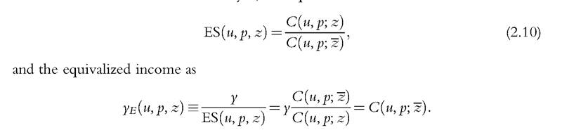
A typical example is the so-called modified OECD scale used by Eurostat, in which the first adult counts for 1, the second adult and each subsequent person aged 14 and over counts for 0.5, and for each additional child under 14 one adds 0.3. The household income is then divided by this scale to get the “equivalized income.”[80] Alternatively, the OECD divides the household income by the square root of the household size. In both cases the reference household (for which the equivalized income equals the original income) is a single. The lack of consensus about the exact scale to be used has also stimulated the use of stochastic dominance approaches (Atkinson and Bourguignon, 1987; Bourguignon, 1989; Fleurbaey et al., 2003; Ooghe and Lambert, 2006). We will not summarize the large literature on equivalence scales here, but rather focus on the differences and similarities with the approaches to measuring well-being that are the topic of this chapter.Using the cost function C(u, p, z) to denote the minimum expenditure needed by a household with characteristics z to reach utility level u if prices are p, and denoting the reference household characteristics by z, the equivalence scale is defined as
By far most attention went to the derivation of equivalence scales on the basis of observed consumption behavior. Traditionally, the analysis of consumption behavior was based on the assumption of a “unitary” household, with preferences and optimization behavior defined at the level of the household. To go beyond the household level and compute individual well-being, it was then commonly assumed that all household members experience the same well-being level. It is clear that in this approach the calculation of equivalence scales requires interpersonal comparisons of well-being between households of different sizes. It is not easy, however, to give an intuitively attractive interpretation to well-being at the level of the household.
More important, it is immediately obvious that consumption data do not yield sufficient information to allow for such interhousehold comparisons of well-being. More specifically, what we can (under some conditions) identify are different sets of indifference curves (one for each household type), but observed consumption does not give us any clue about how to link these indifference curves to utility levels. Stated more formally, the cost functions C(u, p, z) and C(δ(u, z), p, z) will induce exactly the same consumption behavior—where the transformation δ(u, z) may depend on z.Identification of the equivalence scales can only be achieved by introducing additional assumptions. The most famous of these is the so-called IB assumption, where IB stands for “independence of base” (Lewbel, 1989).[81] This assumption states that
the equivalence scale is independent of utility, i.e., C (u, p; z) = C (č, p; z)EB(p, z), where EB(p, z) refers to an equivalence scale that satisfies the IB assumption. This assumption implies a restriction on the cost functions and therefore leads to testable restrictions on the consumption behavior of different households. A crucial part of the identifying assumption is not testable, however, notably the assumption that all households with the same value for y/EB(p, z) indeed reach the same level of utility.
How to interpret this approach in the light of our broader questions about wellbeing? First, the concept of well-being used is a restricted one. In fact, as argued in the short but influential paper by Pollak and Wales (1979), equivalence scales as derived from consumption behavior do not include the direct effects of z on utility—and unless one includes choice of household size in the analysis, choice behavior can never reveal any information about preferences with respect to household size. Pollak and Wales draw a distinction between situation comparisons and welfare comparisons. Situation comparisons are based on the conditional cost function, giving the minimum expenditures needed to reach a given utility level u, conditional on having characteristics z.
Welfare comparisons, on the other hand, require the estimation of an unconditional cost function, giving the minimum expenditures needed to reach a given utility level u, taking into account the direct effect of the characteristics z on utility. In fact, Pollak and Wales are critical of the traditional approach and state that “conditional equivalence scales estimated from observed differences in the consumption patterns of families with different demographic profiles cannot be used to make welfare comparisons” (Pollak and Wales, 1979, p. 220). Unconditional utility (or cost) functions are the representation ofpref- erences over bundles of life dimensions, with household characteristics z as elements of those bundles. Pollak and Wales therefore reject the relevance of traditional equivalence scales and advocate the use of the methods that have been described in the previous sections.Many (or even most) authors studying equivalence scales take a less-negative position and argue that situation comparisons, despite their limitations, are meaningful on their own. They do not yield real welfare comparisons because they do not take into account the direct effect of family life (having a partner and children) on well-being. However, they do make sense in a resource-based approach, focusing on incomes and material consumption only. Some would even claim that inequality in material welfare, as measured by equivalized incomes, is more relevant for policy purposes than inequality in overall well-being, as it is not generally accepted that households should be compensated, e.g., for the fact of having children or not. The relevant question then becomes whether the IB-assumption that the equivalence scale is independent of utility is attractive from a normative point of view. This turns out to be a difficult question as the concepts ofpref- erences and utility are difficult to interpret when applied at the level of the household.
As a matter of fact, this issue extends beyond the problem of correcting for household size.
Similarly, one can calculate equivalence scales for other characteristics z. As an example, Jones and O’Donnell (1995) presented equivalence scales for disability, focusing on “the extra expenditure required by a household with a disabled person to achieve the same level of welfare as a reference household without any disabled individuals.” In such a context of disability, the distinction between situation and welfare comparisons seems even more relevant, although (as noted by the authors) in this setting one can consider these extra expenditures as a lower bound on the welfare loss resulting from disability.A major drawback of the traditional approach is its assumption that preferences and welfare can be defined at the level of the household. It is much more natural to see the household as consisting of individual members, each with their own individual preferences and decidingjointly about household consumption.[82] In this respect, an important recent breakthrough has been the move from the “unitary” to the “collective” model of household behavior (Apps and Rees, 1988; Chiappori, 1988). Some goods are purely private (food or clothing), others are public, and some may be mixed (a car can be used by all household members to make a trip jointly, but it can also be used by only one member of the household). Household resources are allocated to the consumption of each of the household members on the basis of a sharing rule. This rule reflects the relative power positions of the different household members. Finding the restrictions needed to identify the individual preferences of the household members and the sharing rule on the basis of observed consumption behavior in a setting with joint consumption and externalities is a very active and rapidly expanding field of research. This literature is discussed extensively in Chapter 16. Here we focus on the crucial relevance of this work for measuring individual well-being. Indeed, moving from the unitary to the collective model is an important advance in this regard.
A first approach to measuring individual well-being focuses on the sharing rule. If one reasons within a resource-based approach, the share of resources devoted to the consumption of individual i (as influenced by the distribution of power within the household) is an important indicator of his relative well-being level. Identification of the level of the sharing rule is not easy and requires additional restrictions, but Cherchye et al. (2013) show that upper and lower boundaries can be identified in a nonparametric setting. Applying their method to observations in the 1999—2009 Panel Study of Income Dynamics on childless couples, where both adult members participate in the labor market, leads to some interesting insights. As an example, while 11% of their restricted sample have incomes below the two-person poverty line; between 16% and 20% of individuals are below the individual poverty line. Using semiparametric restrictions, Dunbar et al. (2013) identified the resource shares of different household members, including children. Using data for Malawi, they found that the overall poverty rate calculated at the household level understates the incidence of child poverty.
The sharing rule-approach defines well-being in terms of income. For our purposes, another application of the collective approach is more relevant, however. Given that (under some assumptions) it is possible to identify individual preferences, one can formulate an answer to the question: “How much income would an individual living alone need to attain the same indifference curve over goods that the individual attains as a member of the household?” (see, e.g., Browning et al., 2013; Lewbel, 2003). There is an essential difference between this question and the one that was formulated earlier in the context of traditional equivalence scales. To answer this question, one just needs information about the indifference map of the individual, without having to label them. The resulting so-called individual indifference scales are closely related to the notion of equivalent income because they obviously are a form of money-metric utility that can be calculated on the basis of ordinal preference information only. Indifference scales will depend on these preferences, on the “consumption technology” used by the household (in terms of private, public, and mixed goods), and on the sharing rule, i.e., the distribution of power within the household. Applications of this approach have focused, among others, on the adequate compensation in case of wrongful death (Lewbel, 2003) and on poverty among the elderly (Cherchye et al., 2012).
37
Although the introduction of the collective model constitutes an important step forward, it does not bridge the gap between welfare and situation comparisons. Indifference scales do not capture the direct utility effects of partnership and children and remain therefore situated within a resource-based approach. They therefore do not yield a complete measure of well-being taking all relevant life dimensions into account. Whether one considers this to be a problem or not depends on whether one thinks that resource-based (situation) comparisons are relevant from a policy point of view.
Until now, we have discussed the approach to equivalence scales that focuses on observed consumption behavior. Because the focus is on identifying individual preferences, this approach is close to the intuitions underlying the equivalent income approach. Let us now see how the two other approaches to well-being measurement have been applied to tackle the equivalence scales problem.
There are almost no applications within the capabilities framework. Lelli (2005) calculated the equivalence scale of a household with characteristics z as the income needed to reach the same level of functioning (in her case housing) as the reference household. Her application thus remains limited to one functioning—and the resource-based perspective underlying this analysis goes in fact against the basic inspiration of the capability approach.
The subjective (or satisfaction) approach has been used more extensively for the construction of equivalence scales. The pioneering work in this field has been done by Van Praag (1971) and Kapteyn and Van Praag (1976). Originally, these authors assumed that there was a cardinal utility function ofincome U(y; z), where z represents—as before— all relevant nonincome variables. They assumed (on the basis of a theoretical reasoning) that this utility function takes the form ofa lognormal distribution function U(y; μ(yA, z), σ(y, z)), with the mean and the standard deviation dependent on z and on the actual income y of the household. The parameters of that function were estimated on the basis of the answers obtained from what was called the “Income Evaluation Question” (Van Praag, 1971). This question goes as follows:
Please try to indicate what you consider to be an appropriate amount for each of the following cases. Under my (our) conditions I would call a net household income per week/month/year of: about very bad
about___________________________ bad
about___________________________ insufficient
about___________________________ sufficient
about___________________________ good
about___________________________ very good.
Giving specific values to the labels allowed them to estimate the utility function and hence to derive equivalence scales as in expression (10). This original Van Praag approach has never become very popular, partly because of the strong assumptions of cardinality and lognormality.
In later work (e.g., Van Praag and van der Sar, 1988), the cardinality assumption was dropped and the only assumption that was retained was that the different labels (from “very bad” to “very good”) correspond to the same utility values for all individuals (i.e., that they were interpersonally comparable). Denotingthe answers given by individual i for label k by cik, Van Praag and van der Sar (1988) then specified and estimated a (loglinear) function
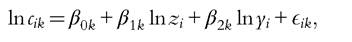
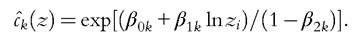
where zi is the size of individual i’s household and Eik is an error term. The coefficients β2k turn out to be highly significant. Respondents with a higher income evaluate the income needed to reach a given utility level as significantly higher than respondents with a lower income. Van Praag talks about a “preference drift” effect, and there is clear echo of the phenomenon of adaptation that has been discussed before. Taking this preference drift into account, one can derive that the “true” cost level needed to reach utility level k is found where
The equivalence scale at level k can then be calculated as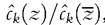 . where z again
denotes the reference household. In their sample of eight European countries and the United States, the equivalence scales are reasonably similar at the different k levels, which gives some support for the IB assumption used in the consumption approach.
Other authors (e.g., Koulovatianos et al., 2005) have implemented a similar method with different formulations of the subjective question. A few papers have combined consumption data and subjective questions (de Ree et al., 2013; Kapteyn, 1994). This is a promising approach because it allows identification of preference parameters on the basis of the subjective information. As an example, de Ree et al. (2013) rejected the IB assumption (and its generalizations) for a sample of Indonesian households.
The question arises of whether the subjective method yields welfare or situation comparisons. Surely, the analyses on the basis of overall life satisfaction that we discussed in the beginning of this section yield welfare comparisons. This is much less clear for the subjective questions used in the literature on equivalence scales, however. Do individuals responding to the income evaluation question take into account the direct effect of household size on well-being? They probably do not, but it is not fully clear for the income evaluation question given earlier. Koulovatianos et al. (2005) confront their respondents with hypothetical household situations and then ask: “Given that someone has an extra child, how much would they need to reach the same level of well-being?” They argue that this yields conditional scales. The subjective information used by de Ree et al. (2013) is even more related to adequacy of resources. The subjective approach to equivalence scales estimation therefore also yields only situation comparisons—and deliberately so.
We can conclude that most of the studies within the equivalence scale approach do not aim at comparisons of well-being, taking into account at the same time the effects of income and of the quality of family life. On the contrary, they aim at needs-corrected values of income, i.e., at conditional comparisons of well-being. They are therefore rooted in a resourcist view on well-being. However, the methods that have been used to calculate equivalence scales are similar to the methods that we described in Section 2.3. The capability approach has hardly been used in this context. Equivalence scales derived from consumption behavior are based on preferences. Although the traditional literature based on the unitary model requires arbitrary assumptions about interpersonal comparability, the recent work with the collective model derives indifference scales using only ordinal preference information. The intuition underlying this approach is closely related to that behind the concept of equivalent income. Subjective evaluations have also been used, and in some of the work there is explicit consideration of the adaptation phenomenon. We will see in the next section that the issue of welfare versus situation comparisons is also relevant to interpret the literature on publicly provided services and benefits.
2.5.2 Publicly Provided Services and Benefits
Countries differ in the extent to which services are provided publicly rather than through the private market, for instance. Comparing the income distribution of two countries, one where health services are primarily covered by private out-of-pocket payments and another where such services are provided free of charge, may result in misleading conclusions on which country is preferable from a social welfare point of view. In addition, publicly provided services and benefits may have an impact on the inequality within a country.[83]
As a starting point, it is fruitful to recall the distinction between functionings and resources. We argued that what matters to define well-being are the functionings of a person, i.e., that person’s “beings” and “doings.” Resources, on the other hand, can be used to achieve certain functionings. These two concepts are different, as individuals may differ in how they convert resources into functionings. An analysis of well-being inequality using a broad set of functionings as the relevant space of well-being includes automatically the publicly provided services, insofar as they contribute to the functionings of the individuals. This approach seems natural in view of the discussions of this chapter. Yet, to the best of our knowledge, examples of this direct method to include publicly provided services into distributional analysis are scarce. Instead, a resource-based approach is standard practice in the literature. In this method, disposable income is extended with a monetary valuation of the publicly provided services. The resulting measure of extended income uses a monetary valuation of the external resources that individuals have at their disposal to obtain functionings and to reach well-being. The inspiration of this approach is therefore closely related to that of equivalence scales as described in the previous section.
In this section, we will first shortly survey the popular approach to extend disposable income with information on publicly provided services. Then we will discuss the issue of the valuation of public services and the adjustment for needs in view of the normative issues discussed in this chapter.[84]
2.5.2.1 The Extended Income Approach
The extended income approach consists of three steps. In a first step, one selects the government services to be included. Then, second, these services are valued at their production cost for the government. Finally, the value of the service is allocated to the beneficiaries based on their actual consumption or the insurance value, depending on the benefit at hand.[85] The obtained value of the monetary value of the publicly provided service is added to the disposable income of the household to obtain its extended income. The distribution of extended income is then analyzed with standard inequality measures.
Applying an extended income approach, the OECD flagship report “Growing Unequal?” (OECD, 2008; Chapter 8) has obtained the following findings. First, the inclusion of publicly provided services reduces income inequality within countries because of their predominantly uniform character. Yet, this reduction is typically lower than the inequality reduction obtained by tax and cash benefits. Second, the differences in income inequality between countries are reduced as well, but the ranking of the countries with respect to extended income inequality remains similar to the ranking according to income inequality (affirming earlier findings of Smeeding et al., 1993).
The extended income approach has the advantage of being implementable for many countries. It requires income data that are readily available in standard household surveys and some additional macroestimates of the production cost of public services. Yet, in view of the normative issues raised in this chapter, the extended income approach appears to take an overly pragmatic view on the valuation of the contribution of publicly provided services to well-being.
2.5.2.2 Valuing Publicly Provided Services and Respect for Preferences
How a publicly provided service should be valued depends arguably on the purpose of the valuation exercise. Whereas valuing the benefit by means of its production cost may give a good estimate of its budgetary cost, this valuation method seems less appropriate for the purpose discussed in this chapter (i.e., an analysis of the distribution of individual well-being).[86]
An example illustrates why this is the case. Imagine that the value of publicly provided education benefits is determined by their production cost. An increase in the wages of teachers increases the production cost, but it seems counterintuitive to say that the value of the service for the recipients has increased because the production cost has increased. Indeed, this valuation method neglects the efficiency of the production process and potential quality differences between equally expensive services. A valuation by means of the production cost can therefore best be seen as an approximation when no other information is available. Alternative valuation methods have been proposed that are more closely related to the preferences of the population.[87]
A first alternative would be to use the market value of the public services rather than the production cost. Under some circumstances market prices may indeed give an indication of willingness-to-pay. Of course, this method can only be applied to the publicly provided services for which a private market exists. For food stamps and social housing, for instance, the market value can either be inferred directly or obtained by a hedonic regression. However, the prices of privately provided services do not always reflect the valuation of the recipients either. Stiglitz et al. (2009, p. 99) give an example in the market for privately provided medical services where informational asymmetries disconnect market prices from marginal valuations and preferences.
A second alternative valuation method relies directly on the preferences of the recipients and measures the value of the publicly provided service by its so-called cash-equivalent. That is the amount of cash needed to induce an individual to forgo a particular publicly provided service (see, Smeeding, 1977, for instance). Insofar as the individual’s own preferences (her own willingness-to-pay) are used to compute these cash equivalents, this method respects the same-preference principle. Figure 2.6 illustrates the cash-equivalent valuation method graphically in the income-health space. Consider two individuals, Alexandra and Benny, who are equally rich (their income equals OA on the graph). Alexandra is in better health than Benny (their health is respectively OG and OE). Both individuals receive publicly provided health services, without which Alexandra’s health would be OF, whereas Benny’s health would be only OD. It is clear from the figure that the publicly provided health services generate a larger increase in the health of Benny than they do for Alexandra. However, Benny cares relatively less about his health than Alexandra does (as Benny’s indifference curve is “steeper”). Benny’s cash equivalent for the health service is AB, as Benny is willing to forgo the publicly provided health service for an additional income of AB. Alexandra’s cash equivalent, on the other hand, equals AC. Even if the health service generates a smaller health increase for Alexandra, her cash equivalent is larger, as she cares more about health than Benny does.
Estimating a cash equivalent requires additional information compared to the production cost approach. As illustrated by the preceding example, one needs to know the preferences of Alexandra and Benny because the magnitude of their cash equivalent is determined by the shape of their indifference map. To obtain the necessary information on preferences, the methods surveyed in Section 2.3 can be used, i.e., revealed preferences, stated preferences, and satisfaction data. The revealed preferences method seems to be favored in the applied literature. Typically, the preferences are derived from consumption behavior by means of an estimated system of demand equations (Slesnick, 1996; Smolensky et al., 1977). Life satisfaction data can also be used to estimate willingness- to-pay for publicly provided services. Levinson (2012), for instance, estimated the willingness-to-pay for air quality and computes the compensating variation for air pollution.
Typically the cash-equivalent method is not formulated in the space of functionings (or life dimensions), and it does not yield an overall measure of well-being that is based on a coherent ethical reasoning. We will come back to this issue in the following subsection. However, because it focuses on the individual willingness-to-pay, its inspiration remains
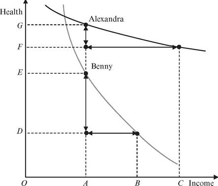
Figure 2.6 Cash equivalent income.
similar to that of the equivalent income approach to well-being as defined in Section 2.3.3. Other approaches reject completely the idea that individual preferences and willingness-to-pay provide the best guidelines to value publicly provided services.
Governments may provide these in-kind services exactly because they are inspired by paternalistic motives or by a concern about consumption externalities (see Currie and Gahvari, 2008, and the references therein for a detailed discussion). The paternalistic motivations reflect Musgrave’s (1959) idea that some goods are merit goods, which leads to an immediate conflict with the idea of respecting individual preferences. A paternalistic government values the publicly provided services according to an objective valuation function, which requires arguably a perfectionist or objective theory of well-being. As suggested before, the gap between these two approaches may be bridged to some extent by introducing a distinction between informed and uninformed preferences.
2.5.2.3 Adjusting for Needs and Individual Responsibility
Because extended income focuses on the willingness-to-pay for the services, it does not at all take into account the functioning levels that the individuals would obtain in absence of any publicly provided service. This can be seen using Figure 2.7, depicting the functionings and indifference curves of Alexandra and Charlotte in the income-health space. Alexandra and Charlotte have the same income (OA) and obtain the same increase in their health from the publicly provided health services (ED = FG). Moreover they have the same preferences, so their cash equivalents are equal to AC.[88] Hence, the extended income of both individuals is equal (OC). Consequently, when extended income would be used as a measure of well-being, both individuals would be considered as equally well off.Yet, no account is taken of the fact that the health levels that the individuals would obtain in absence of any publicly provided health service may be very different (Alexandra is in much better health than Charlotte, OF > OD). Radner (1997) illustrated a similar issue by showing how the well-being of elderly (Charlotte in Figure 2.7) would be overestimated as the value of publicly provided services is included in their extended income without taking account of their needs. This observation led Paulus et al. (2010, p. 263) to doubt whether results derived using the extended income approach can have a straightforward welfare interpretation.
43
This discussion echoes the distinction that was introduced in the previous section between welfare and situation comparisons. As a matter of fact, in the recent applied literature, the solution has been sought in adjusting the equivalence scales of the recipients for differences in needs.[89] Paulus et al. (2010) adopted a “fixed cost” approach, in which the needs of a recipient are assumed to be equal to a specific fixed monetary amount. In particular, it is assumed that the per capita amounts spent for age-specific population groups on public services accurately depict the corresponding needs of these groups. Under this assumption an equivalence scale for extended income can be inferred for each household. The authors then performed a sensitivity analysis of the inequality reducing
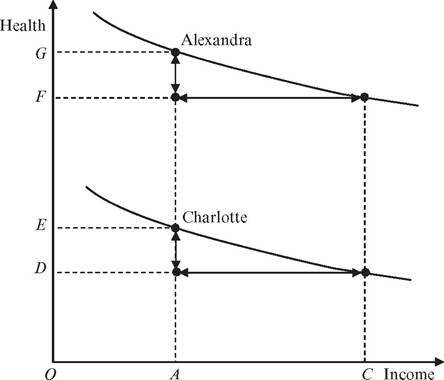
Figure 2.7 Cash equivalent income and needs.
effect of public services from changing the amount of received publicly provided services to the European average for the age-specific groups.
Aaberge et al. (2010) derived needs-adjusted equivalence scales consistent with their preferred allocation method of the production costs across target groups (i.e., a model of spending behavior of local governments). The equivalence scale for noncash income is obtained from the estimates of the relative needs of different target groups that are derived from the minimum expenditures identified in the spending model. Using data from Norway, they find that including publicly provided services reduces income inequality considerably, but that adjusting for needs offsets about half of the inequality reduction.
The method hinges on two strong assumptions on the interpretation of the spending model for the local governments (Aaberge et al., 2010, p. 552). First, the estimated minimum expenditures are to be interpreted as originating from an implicit consensus among local governments about how much spending the different target groups need minimally. Second, the functional form of the individual well-being measure derived from public services is assumed to coincide with the functional form used by local governments to decide the spending on public services. A priori, it seems hard to square such a (heroic) assumption with the idea of respecting individual preferences.
Both approaches to compute a needs-adjusted extended income rely on a two-step procedure. In a first step, the extended income is computed by adding a monetary value of the publicly provided services to the disposable income of the individual. Then, in a second step, these extended incomes are adjusted for differences in individual needs by means of an equivalence scale. A natural alternative would be to measure well-being directly in the desired space, i.e., functionings or capabilities themselves. For that purpose, a well-being measure should be developed along the lines described in Section 2.3 of this chapter. The relationship between these broader measures and the resource-based measures that are used now deserves a deeper exploration.
2.5.3 International Comparisons
The international comparison of living standards is fraught with many difficulties (see also Chapter 11). Because the focus in this literature has often been on comparing real incomes, we will first discuss the difficulties related to differences in prices for market commodities, and we will show how they are linked to the normative issues discussed in the previous sections. We will then show the relevance of introducing nonmarket dimensions into the evaluation of living standards.
2.5.3.1 PPP Indexes
International comparisons of living standards involve the search for price deflators that make it possible to compute comparable real incomes.[90] Pragmatic convenience
45
motivates approaches in which indexes are computed directly from prices and quantities, without depending on an estimation of consumer preferences. The theory of index numbers initiated by Fisher (1922) and developed by Diewert (1976,1992a,b) is an important source of inspiration for such indexes. Pragmatic convenience also encourages seeking formulae that make the comparison of two countries independent of data from third countries.
Consistency is akin to transitivity in the comparison of real incomes, but a cardinal form of transitivity (involving orders of magnitude) appears desirable, not just an ordinal form. For instance, if Qij is a quantity index that compares real income in country i to country j, consistency is achieved when the chain relation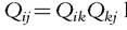 holds for every
third country k. A popular way of achieving consistency computes real income as the value of quantities consumed at reference prices p, so that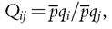 where qi is
the vector of total consumption in country i.
All approaches have a connection with consumer preferences, but the conditions required are more or less restrictive, and the connection therefore more or less loose. There seems to be near consensus, in the PPP literature, that “in so far as data on real income have any meaning, it is that they provide an answer to the question: ‘How well off would the same reference consumer be in different countries?’” (Neary, 2004, p. 1425). In other words, even if heterogeneous preferences may be the fact of the matter, there is no real attempt to formulate indexes that reflect this diversity of preferences. The main implicit underlying argument seems to be that ordinal preferences do not allow for interpersonal comparisons, unless arbitrary assumptions are made. In particular, money-metric utilities are not considered a possible option, although very similar notions are sometimes used, as explained later. This observation again suggests that the focus is not on welfare comparisons, but on situation comparisons.
Let us first briefly describe the two most popular PPP methodologies. The Elteto- Koves-Szulc (EKS) quantity indices, used by the OECD and Eurostat are multilateral extensions of the Fisher index:
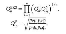
They satisfy consistency in the form of the chain relation, but depend on third country data. They do not require estimation of preferences, and the link to consumer preferences isusually made by referring to Diewert’s (1976) argument that the Fisher quantity index  is equal to the exact index
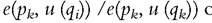 >f a flexible expenditure function e
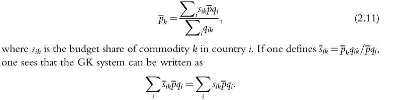
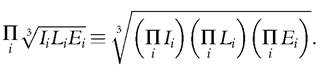
(p, u), i.e., a function that approximates any twice differentiable expenditure function to the second order. Along a similar vein, Neary (2004) proved that Another popular approach, used by the U.N. International Comparison Project and the Penn World Table (PWT), relies on the Geary-Khamis (GK) indices, which compute PPP expenditures as the value of consumption at reference prices,and the reference prices are derived from the system This approach obviously satisfies consistency. It depends on third country data, but only in the computation ofp. The link with consumer preferences is tenuous because pqi provides a good index only for Leontiefpreferences (which would imply that all countries’ consumption vectors should be proportional to one another). Neary (2004) then proposed, as a variant, to estimate world consumer preferences and substitute compensated Interestingly, nothing in expression (11) as modified by Neary requires identical preferences, so that one could apply Neary’s methodology to a population with countryspecific estimated preferences, in which case the real incomes be money-metric utilities at the country level. This idea is not considered in van Veelen and van der Weide (2008) or in the reply by Crawford and Neary (2008). As mentioned earlier, Fleurbaey and Blanchet (2013) proposed to take other reference prices van Veelen (2002) proved an impossibility theorem that is similar to the incompatibility between the personal-preference principle and the dominance principle discussed earlier in this chapter. This theorem says that there is no measure of real income (based on prices and quantities in all countries) that is continuous, is not independent of prices, satisfies dominance (qi > qj∙ implies that real income is greater in i), and such that pairwise comparisons are independent of third countries.4 The EKS and GK methods satisfy all conditions except the last one. A money-metric approach that estimates preferences on the same data may, in addition, fail to satisfy dominance in the case of heterogeneous estimated preferences. We know that this is a necessary consequence of respecting heterogeneous preferences.[93] [94] In a recent paper, Almas (2012) considers exploiting preference data by estimating budget coefficients with household surveys, but retains the assumption of identical preferences. Instead of estimating a complete system of demand functions to compute expenditure functions and money-metric utilities, she focused on food and assumed that the equation of food share, conditional on demographic characteristics, is the same everywhere. Estimating it with the PPP price indexes from the PWT, she included country dummies and assimilated these dummies to a bias in the PPP indices. This method relies on the assumption that preferences for food versus other goods are identical all over the world, and it is not indicative of welfare because incomes deflated with the corrected indices are not money-metric utilities for the AIDS model that is estimated.[95] Deaton (2010) and Deaton and Heston (2010) studied the difficulties created by the fact that different countries in fact consume different lists of commodities, with great differences between countries with very unequal standards of living. The worst configuration would, of course, be the case in which every country consumes its own specific list, that has no intersection with the list of other countries. In this case, it is hard to imagine how to perform comparisons on the basis of observed market demand data. But even when all pairs of countries have a nonempty intersection of lists, the imperfect overlap creates difficulties. Practical methods that single out identical but often nonrepresentative goods appear unsatisfactory (a popular example, however, is the so-called Big Mac Index, published yearly by the Economist). Using proximate countries to compute chained indexes may lead to compounding errors as one compares distant countries. Deaton (2010) suggested that nondemand data, such as well-being questionnaires, may provide useful additional information for comparisons across countries. On the theory side, Fleurbaey and Tadenuma (2007) showed that imperfect overlap of commodity lists generates Arrow-like impossibility theorems, even if one only relies on the weak independence axiom stipulating that the evaluation of two allocations should only depend on preferences over the commodities that appear in either allocation. As a way out, they suggested focusing on lists of functionings that have a common set of core components, which is not very different from Deaton’s suggestion to go beyond market data. Of course, these suggestions immediately bring us the more general topic of introducing nonmarket dimensions. 2.5.3.2 Nonmarket Dimensions The recognition that living standards incorporate public goods of many sorts (e.g., the environment), as well as nonmarketed goods and “functionings” (e.g., health), has played an important role in the motivation to go “beyond GDP” not just for the evaluation of growth and public policy in a given country, but also in international comparisons. In fact, all three approaches that were reviewed in Section 2.3 have been applied in empirical work on intercountry comparisons. The simplest approach consists in aggregating indices of the different dimensions of life into a single composite indicator. This approach follows the objective interpretation ofthe capability approach. The most popular example is the HDI that aggregates three indices (which are normalized between 0 and 1 from the range of achievements by the various countries of the world): national income, life expectancy, and education. Although the initial version of the index made a linear aggregation (UNDP, 1990) and therefore implied perfect substitutability between the dimensions, the geometric mean has recently been adopted to reflect the greater importance of a dimension when its level is low compared to the others (UNDP, 2010). In a variant of the new index, the average indices per domain can be adjusted for inequality, so as to make each index a geometric mean of individual achievements. In this fashion, the global index can then also be written as the geometric mean of individual Cobb-Douglas indexes, due to the following identity (where Ii, Li, Ei denote income, life expectancy, and education for individual i): This variant alleviates the criticism raised against specific composite well-being indicators, that they fail to take the correlations between the dimensions or cumulative deprivation into account as they start from dimension-by-dimension summary statistics (see Section 2.4). In the preceding formula, the same elasticity of substitution is applied in the aggregation across dimensions and across individuals, so that the sequencing of both aggregations does not matter. This makes the index impervious to correlations between dimensions. Moreover, the present version of the HDI is clearly an objective index which—according to some—implies troubling trade-offs between the dimensions (see Ravallion, 2012, for instance). There are many composite indicators that mimic the HDI methodology.[96] Some focus on social issues, whereas others focus on sustainability issues. The key difficulty for such indices is the choice of the weighting system for the various dimensions. It is quite common to perform sensitivity analysis to ascertain the robustness of conclusions to the weights (Decancq and Ooghe, 2010; Foster et al., 2013), which boils down to a dominance analysis. Another approach is to give up the aggregate index altogether and immediately apply multidimensional inequality indices to the same data (Decancq et al., 2009). Of course, as we saw in Section 2.4, none of these approaches allows to respect international preference heterogeneity. The happiness approach has also been used for international comparisons, although much of the literature on cross-country data has focused on the link between happiness and income (Deaton, 2008; Diener et al., 2010; Stevenson and Wolfers, 2008). The great variations in average satisfaction with life at any given level of income may reflect differences in nonmarket dimensions of life, but also cultural variations. Helliwell et al. (2010) studied a large sample of countries and derived two conclusions. First, nonmarket dimensions play a large role in econometric regressions of life satisfaction. Such dimensions include having a partner, being able to count on friends, having freedom to choose, not perceiving corruption around oneself, having been generous, and practicing religion. These dimensions play a role at the individual level, but for some of them the national average also plays a role (including healthy life expectancy, which is not observed at the individual level). The second conclusion is that once one incorporates these social dimensions in the analysis, in a single equation of satisfaction with the same coefficients for all countries, the difference between predicted and actual values for the average level of satisfaction per country is small for most countries and has no systematic pattern, with one exception: the Latin-American countries in general have a higher well-being than predicted. However, the results of country and regional equations also show that the coefficients of income and social dimensions vary substantially, revealing that the association between life satisfaction and the various dimensions of life is heterogeneous over the world. One can suspect that interpersonal heterogeneity may be even more important. If the satisfaction equations can be interpreted as giving some evidence on population preferences, this raises the interesting issue of comparing the situations of populations with different preferences—an issue that has been central in this chapter. Helliwell et al. (2010) proposed to compute income equivalent variations via the ratios of coefficients of social dimensions over the income coefficient. This method is one of those that have been introduced in Section 2.3 to estimate preferences necessary to calculate equivalent incomes. 51 The method of income equivalent variations has been used by Becker et al. (2005) to estimate the income growth that would have been equivalent to the observed increase in life expectancy for various countries of the world. Their main finding is that the large increase in life expectancy in developing countries, once converted into a monetary equivalent, produces a much rosier picture of world inequalities than standard income measures. They assumed homogeneous preferences in the world, and their estimation of preferences relied on U.S. data on revealed preferences about job risks. A combination of equivalent variations and compensating variations has been used by Jones and Klenow (2010), with a preference relation similar to that used in Becker et al. (2005), but extending the list of nonincome dimensions to include leisure time and inequalities. Letting I and Q denote income and quality of life (life expectancy, leisure, inequalities) and V a utility function representing the preference ordering (assumed to be common across countries), the equivalent variation approach solves the following equation, for each country i: while the compensating variation approach solves the equation They then propose to take A difficulty with the compensating variation approach, as they implement it, is that Compensating and equivalent variation approaches are in general problematic when they make references vary with the object of comparison. Money-metric indexes avoid that difficulty by taking a fixed reference. Fleurbaey and Gaulier (2009) adopted a money-metric approach for international comparisons of OECD countries, with nonincome dimensions including leisure, life expectancy, unemployment risk, household composition, and income inequalities. They allowed for heterogeneous preferences for leisure only and relied on the Becker et al. (2005) preference ordering otherwise. Although the approach is in theory compatible with heterogeneous preferences at the individual level and the computation of a distribution of equivalent incomes within each country, they only focused on average levels for each country. Decancq and Schokkaert (2013) calculated individual equivalent incomes on the basis of the life satisfaction data from the European Social Survey with as nonincome dimensions health, employment status, quality of social interactions, and personal safety. They introduced these equivalent incomes into a concave social welfare function and compared the social welfare of 18 European countries for the years 2008 and 2010, taking into account the distribution of individual well-being. The ranking of the different countries in terms of equivalent incomes is different from the ranking of countries in terms of income. A striking example is the dramatic fall in the well-being of Greece and Spain as a result of the economic crisis. Bargain et al. (2013) studied heterogeneous preferences over consumption and leisure in various European countries and the United States and computed several money-metric indexes for the analysis of welfare level and inequalities. In their analysis also, preference heterogeneity plays an important role in the welfare rankings. 2.6.
 is equal to the ratio of utilities when utility is quadratic
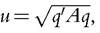 for some suitably chosen symmetric matrix A. Again, a quadratic utility is a flexible form. These approximation results, however, are compatible with the index being sometimes wrong in the first order even for small changes—as must happen with any index that ignores preferences.[91] [92]
 preferences—but not necessarily to the population’s actual preferences if they are heterogeneous, as noted in van Veelen and van der Weide (2008).
 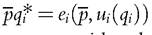 would
would 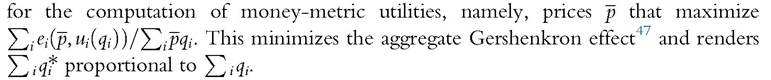
 as the index for comparisons across countries.
  of life in the United States as the reference.
More on the topic APPLICATIONS:
- Choosing between different environmental policy instruments
- Models for J0 and J
- Alsharari Nizar Mohammad (ed.). Banking and Accounting Issues. ITexLi,2022. — 175 p., 2022
- Contents
- Qatar
- The inquiry on al-ta'adul wa-l-tarjih or al-ta‘arud wa-l-tarjih in Islamic theoretical jurisprudence addresses, in general terms, what jurists should do when they encounter in their legal research what appear to be conflicting arguments of equal strength.
- Conclusion
- Maldives