Applications of Stochastic Dynamic Programming
We now present a number of applications of the methods of stochastic dynamic programming. Some of the most important applications, related to stochastic growth and growth with incomplete markets, are left for next chapter.
In each application, I try to point out how formulating the problem recursively and using stochastic dynamic programming methods simplify the analysis.16.5.1. The Permanent Income Hypothesis. One of the most important applications of stochastic dynamic optimization is to the consumption smoothing problem of the consumer facing an uncertain income stream. This problem was first discussed by Irving Fisher (1930) and then received its first systematic analysis in Milton Friedman’s classic book on consumption theory (1956). With Robert Hall’s (1978) seminal paper on dynamic consumption behavior it became one of the most celebrated macroeconomic models. Here I present a simple version of this problem with linear-quadratic preferences and characterize the solution using the sequence formulation of the problem and also stochastic dynamic programming.
Consider a consumer maximizing discounted lifetime utility
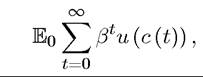
with c (t) ≥ 0 as usual denoting consumption. To start with we assume that u (∙) is strictly increasing, continuously differentiable and concave and denote its derivative by u0 (∙). We will shortly look at the case in which u (∙) is given by a quadratic.
The consumer can borrow and lend freely at a constant interest rate r > 0, thus his lifetime budget constraint takes the form
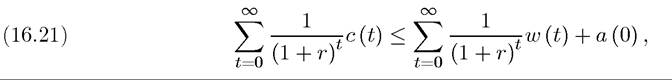
where a (0) denotes his initial assets and w (t) is his labor income. We assume that w (t) is random and takes values from the set W ? {wi,...,wn}.
This corresponds to potential labor income fluctuations due to aggregate or idiosyncratic shocks facing the individual. To simplify the analysis, let us suppose that w (t) is distributed independently over time and the probability that w (t) = wj is qj (naturally with Consequently, the lifetime
 budget constraint (16.21) has to be interpreted as a stochastic constraint. We therefore require this constraint to hold almost surely. This implies that the constraint has to hold with probability 1. The reader may wonder why this particular concept from measure theory has crept into our discussion, since w (t) still takes finitely many values. The reason is that even when w (t) takes only finitely many values, the probability distribution for the infinite sequence of random variables w∞ ? (w (0),w (1),...) is equivalent to a continuous probability distribution. Nevertheless, for our purposes this is also a technicality and not much more than the requirement that the lifetime budget constraint (16.21) should hold almost surely is necessary for our analysis.
Leaving technicalities aside, the fact that the lifetime budget constraint is stochastic has important economic implications. In particular, although we have not introduced an explicit borrowing constraint, the fact that the lifetime budget constraint must hold with probability 1 imposes endogenous borrowing constraints. For example, suppose that wι = 0 and qi > 0 (so that this state corresponds to unemployment and zero labor income). Then there is a positive probability that the individual will receive zero income for any sequence of periods of length T < ∞. Then if the individual ever chooses a negative asset holding, a (t) < 0, there will be a positive probability of violating his lifetime budget constraint, even if he were to choose zero consumption in all future periods. Therefore, there is an endogenous borrowing constraint, which takes the form
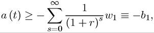
with wι denoting the minimum value of w within the set W and the last relationship defining bi.
Let us first solve this problem treating it as a sequence problem, that is, the problem of choosing a sequence of feasible plans This can be done simply by forming
a Lagrangian. Even though there is a single lifetime budget constraint (16.21), it would be incorrect to treat the problem as if there were a unique Lagrange multiplier λ. This is because consumption plans are made conditional on the realizations of events up to a certain date. In particular, consumption at time t will be conditioned on the history of shocks up to that date, wt ? (w (0),w (1),...,w (t)), and in fact we use the notatior to emphasize that consumption at date t is a mapping from the history of income realizations, wt. At that point, since there is also more information about how much the individual has earned and how much he has spent, it is also natural to think that the Lagrange multiplier, which represents the marginal utility of money, is also a random variable and can depend only on the realizations of the shocks up to date t, wt. We therefore write this multiplier as
The first-order conditions for this problem immediately give

which requires the (discounted) marginal utility of consumption after history wt to be equated to the (discounted) marginal utility of income after history While economically
interpretable, this first-order condition is not particularly useful unless we know the law of motion of the marginal utility of income This law of motion is not straightforward to derive with this formulation.
prices for all possible claims to consumption contingent on any realization of history are introduced, is much more tractable and gives similar results to the recursive approach below. I will introduce this contingent-claims formulation in the analysis of the competitive equilibrium of the neoclassical growth model under uncertainty in the next chapter.
Instead, if we formulate the same problem recursively, sharper results can be easily obtained. Using the tools of this chapter, let us write this problem recursively. First, instead of the lifetime budget constraint, the flow budget constraint of the individual can be written as 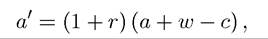 where a' refers to next period’s asset holdings. Conversely, this implies
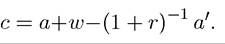
Then the value function of the individual, conditioned on current asset holding a and current realization of the income shock w, can be written as

where I have made use of the fact that w is distributed independently across periods, so the expectation of the continuation value is not conditioned on the current realization of w. Now as in Example 6.5 in Chapter 6, where we studied the non-stochastic version of this problem, 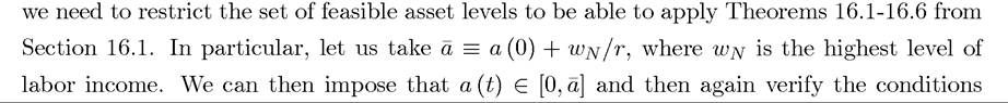 under which this has no effect on the solution (in particular the condition for a (t) to be always in the interior of the set, see Exercise 16.10).
The first-order condition for the maximization problem gives
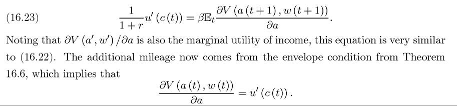
Combining this equation with (16.23), we obtain the famous stochastic Euler equation of stochastic permanent income hypothesis:

The notable feature here is that on the right-hand side we have the expectation of the marginal utility of consumption at date t + 1.
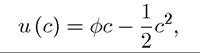
We thus have a simple stochastic Euler equation.This equation becomes even simpler and perhaps more insightful when we assume that the utility function is quadratic, for example, taking the form
633
with φ sufficiently large that in the relevant range u (∙) is increasing in c. Using this quadratic form with (16.24), we obtain Hall’s famous stochastic equation that

where κ ? β (1 + r). A striking prediction of this equation is that variables, such as current or past income, should not predict future consumption growth. A large empirical literature investigates whether or not this is the case in aggregate or individual data, focusing on excess sensitivity tests. If future consumption growth depends on current income, this is interpreted as evidence for excess sensitivity, rejecting (16.25). This rejection is often considered as evidence in favor of credit constraints, which prevent individuals from freely borrowing and lending (subject to the endogenous borrowing constraint derived above). Nevertheless, excess sensitivity can also emerge when the utility function is not quadratic (see, for example, Zeldes, 1989, Caballero, 1990).
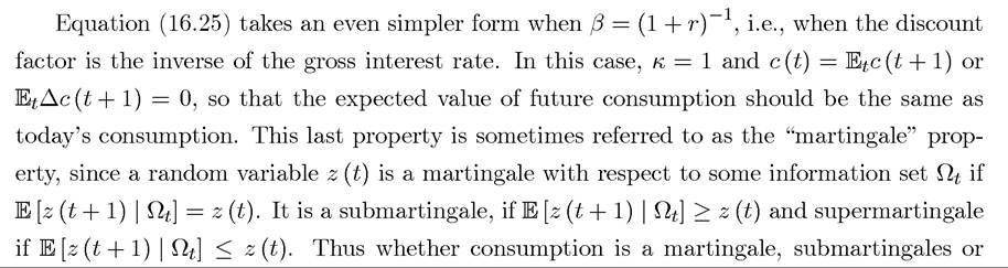
supermartingale depends on the interest rate relative to the discount factor. Exercises 16.7 and 16.10 further discuss the implications of this equation.
16.5.2. Search for Ideas. This subsection provides another example of an economic problem where dynamic programming techniques are very useful. This example also provides us with an alternative and complementary way of thinking about the endogeneity of technology to that offered by the models presented in Part 4.
Consider the problem of a single entrepreneur, with risk-neutral ob jective function
This entrepreneur’s consumption is given by the income he generates in that period (there is no saving or borrowing).
The entrepreneur can produce income equal to
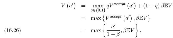
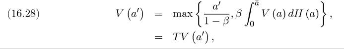
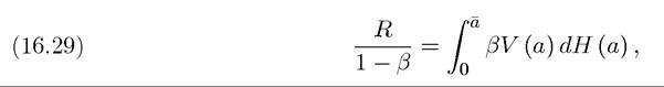
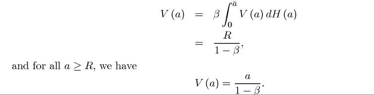
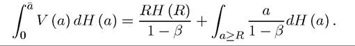
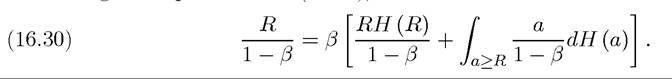
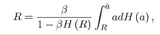
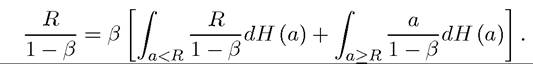
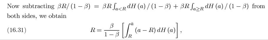
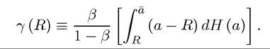
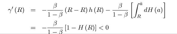
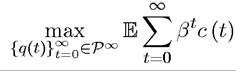
at time t, where t = 0, the entrepreneur starts with a (0) = 0. From then on, at each date, he can either engage in production using one of the techniques he has already discovered, or spend that period searching for a new technique. Let us assume that each period in which he engages in such a search, he gets an independent draw from a time-invariant distribution function H (a) defined over a bounded interval [0, d]. Therefore, the decision of the entrepreneur at each date is whether to search for a new technique or to produce with one of the techniques he has discovered so far. The consumption decision of the entrepreneur is trivial, since there is no saving or borrowing, and he has to consume his current income, c(t) = y (t). This problem introduces a slightly different perspective on some of the ideas already discussed in the book. In particular, as in the endogenous technological change models we have studied so far, the entrepreneur has a non-trivial choice which affects the technology available to him; by searching more, which is a costly activity in terms of foregone production, he can potentially improve the set of techniques available to him. Moreover, this economic decision is related to the standard tradeoffs in technology choices; whether to produce with what he has available today or make an “investment” in one more round of search with the hope of discovering something better. This type of economic tradeoff is complementary to the incentives to invest in new technology in the models of endogenous technology we have already seen in the previous part of the book. For now, our main objective is to demonstrate how dynamic programming techniques can be used to analyze this problem. Let us first try to write the maximization problem facing the entrepreneur as a sequence problem. We begin with the class of decision rules of the agent. In particular, let entrepreneur over the past t periods, with a (s) = 0, if at time s, the entrepreneur engaged in production. We write which denotes the action of the agent at time t, which is either to produce with the current technique he has discovered, a (t), or to choose q (t) = “search” and spend that period searching for or researching a new technique. Let Pt be the set of functions from At into a (t) U {search}, and P∞ the set of infinite sequences of such functions. The most general way of expressing the problem of the individual would be as follows. Let E be the expectations operator. Then the individual’s problem is subject to c (t) = 0 if q (t) = “search” and c (t) = a0 if q (t) = a0 for a (s) = a0 for some s ≤ t. Naturally, written in this way, the problem looks complicated, even daunting. The point of writing it in this way is to show that in certain classes of models, the dynamic 635 Introduction to Modern Economic Growth programming formulation will be quite tractable even when the sequence problem may look quite complicated. To demonstrate this, we now write this optimization problem recursively using dynamic programming techniques. Let us simplify the formulation of the recursive form of this problem by making two observations (which will both be proved in Exercise 16.11). First, because the problem is stationary we can discard all of the techniques that the individual has sampled except the last one and thus write the problem simply conditioning on the last period’s stochastic state. In particular, denote the value of an agent who has just sampled a technique Therefore, we can write where q is the acceptance decision, with q = 1 corresponding to acceptance, and is the expected continuation value of not producing at the available techniques. The expression in (16.26) follows from the fact that the individual will choose whichever option, starting production or continuing to search, gives him higher utility. That the value of continuing to search is given by (16.27) follows by definition. At the next date, the individual will have value V (a) as given by (16.26) when he draws a from the distribution H (a), and thus integrating over this expression gives EV. The integral is written as a Lebesgue integral, since we have not assumed that H (a) has a continuous density. A SLIGHT DIGRESSION*. Even though the special structure of the search problem enables a direct solution, it is also useful to see that optimal policies can be derived by applying the techniques developed in Section 6.3 in Chapter 6. For this, combine the two previous equations and write where the second line defines the mapping T. Now (16.28) is in a form to which we can apply the above theorems. Blackwell’s sufficiency theorem (Theorem 6.9) applies directly and implies that T is a contraction since it is monotonic and satisfies discounting. Next, let V ∈ C ([0, a]), i.e., the set of real-valued continuous (hence bounded) functions defined over the set [0, a], which is a complete metric space with the sup norm. Then the Contraction Mapping Theorem, Theorem 6.7 from Chapter 6, immediately implies that a unique value function V (a) exists in this space. Thus the dynamic programming formulation of the sequential search problem immediately leads to the existence of an optimal solution (and thus optimal strategies, which will be characterized below). Moreover, Theorem 6.8 also applies by taking S' to be the space of nondecreasing continuous functions over [0, a], which is a closed subspace of C ([0, d]). Therefore, V (a) is nondecreasing. In fact, using Theorem 6.8 we could also prove that V (a) is piecewise linear with first a flat portion and then an increasing portion. Let the space of such functions be S'', which is another subspace of C ([0, d]), but is not closed. Nevertheless, now the second part of Theorem 6.8 applies, since starting with any nondecreasing function V (a), TV (a) will be a piecewise linear function starting with a flat portion. Therefore, the theorem implies that the unique fixed point, V (a), must have this property too. ■ The digression above used Theorem 6.8 from Chapter 6 to argue that V (a) would take a piecewise linear form. In fact, in this case, this property can also be deduced directly from (16.28), since V (a) is a maximum of two functions, one of them flat and the other one linear. Therefore V (a) must be piecewise linear, with first a flat portion. Our next task is to determine the optimal policy using the recursive formulation of Problem B2. The fact that V (a) is linear (and strictly increasing) after a flat portion immediately tells us that the optimal policy will take a cutoff rule, meaning that there will exist a cutoff technology level R such that all techniques above R are accepted and production starts, while those a < R are turned down and the entrepreneur continues to search. This cutoff rule property follows because V (a) is strictly increasing after some level, thus if some technology a' is accepted, all technologies with a > a' will also be accepted. Moreover, this cutoff rule must satisfy the following equation 637 so that the individual is just indifferent between accepting the technology a = R and waiting for one more period. Next we also have that since a < R are turned down, for all a < R Using these observations, we obtain Combining this equation with (16.29), we have Manipulating this equation, we obtain which is a convenient way of expressing the cutoff rule R. Equation (16.30) can be rewritten in a more useful way as follows: which is an important way of characterizing the cutoff rule. The left-hand side is best understood as the cost of foregoing production with a technology of R, while the right-hand side is the expected benefit of one more round of search. At the cutoff threshold, these two terms have to be equal, since the entrepreneur is indifferent between starting production and continuing search. Let us now define the right-hand side of equation (16.31), the expected benefit of one more search, as Suppose also that H has a continuous density, denoted by h. Then we have 638 This implies that equation (16.31) has a unique solution. It can be easily verified that a higher β, by making the entrepreneur more patient, increases the cutoff threshold R. 16.5.3. Other Applications. There are numerous other applications of stochastic dynamic programming. In addition to the three growth models we will study in the next chapter, the following are noteworthy. (1) Asset Pricing: following Lucas (1978), we can consider an economy in which a set of identical agents trade claims on stochastic returns of a set of given assets (“trees”). Each agent solves a consumption smoothing problem similar to that in subsection 16.5.1, with the major difference that he or she has to save in assets with stochastic returns rather than at a constant interest rate. Market clearing will be achieved when the total supply of assets is equal to total demand. This implies that in equilibrium the prices have to be such that each agent is happy to hold the appropriate amount of claims on the returns from these assets. Given the marginal utility of consumption derived from the recursive formulation, these assets can be priced. Exercise 16.13 considers this case. (2) Investment under Uncertainty: the model of investment under adjustment costs discussed in Section 7.8 of Chapter 7 has much wider application in macroeconomics and industrial organization once augmented by the possibility that firms are uncertain about future demand and/or productivity. Exercise 16.14 considers this case. (3) Optimal Stopping Problems: the search model discussed in the previous subsection is an example of an optimal stopping problem. More general optimal stopping problems can also be set up and analyzed as stochastic dynamic programming problems. Exercise 16.15 considers an example of such a stopping problem. 16.6.
 is the quality of the technique he has available for production.[34] [35] At
  be a sequence of techniques observed by the
  Then a decision rule for this individual would be
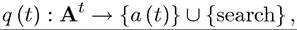

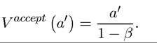
 Second, we suppose that once the individual starts producing at some technique a', he will continue to do so forever, instead of going back to searching again at some future date. This is also intuitive due to the stationarity of the problem; if the individual is willing to accept production at technique a' rather than searching more at time t, he would also do so at time t +1. This last observation implies that if the individual accepts production at some technique a' at date t, he will consume c (s) = a' for all s ≥ t. Consequently, we obtain the value on accepting technique a0 as