Generalization to Markov Processes*
What happens if z does not take on finitely many values? For example, z may be represented by a general Markov process, taking values in a compact metric space. The simplest example would be a one-dimensional stochastic variable z (t) given by the process z (t) = ρz (t — 1) + σε (t), where ε (t) has a standard normal distribution.
At some level, most of the results we care about generalize to such cases. At another level, however, greater care needs to be taken in formulating these problems both in the sequence form of Problem B1 and in the recursive form of Problem B2. The main difficulty in this case arises in ensuring that there exist appropriately defined feasible plans, which now need to be “measurable” with respect to the information set available at the time. Unfortunately, to state the appropriate theorems in a rigorous manner requires a lengthy detour into measure theory. Instead, I will assume that both Z and X are compact and that the function introduced in Section 16.1 is “well-defined”—in particular, finite-valued and measurable. Under these assumptions and again representing all integrals with the expectations, we can state the main theorems for stochastic dynamic programming with general Markov processes without proof.
 Let us first define Z as a compact subset of R, which includes Z consisting of finite number of elements and Z corresponding to an interval as special cases. Let z (t) ∈ Z represent the uncertainty in this environment, and suppose that its probability distribution can be represented as a Markov process, i.e.,

Let us also use the notation to represent the history of the realiza
tions of the stochastic variable.
The objective function and the constraint sets are represented as in Section 16.1, so that again denotes a feasible plan. Let the set of feasible plans after history zt be denoted by
 . The set of feasible plans starting with
  is then
 Also whenever there exists a function V that is a solution to
Problem B2, let us define Π (x, z) ⊂Φ(x, z) such that any π (x, z) ∈ Π (x, z) satisfies

Finally, to state the appropriate theorems, let us refer to the same assumptions as in Section 16.1, except that these assumptions now require the relevant functions to be measurable in the appropriate sense and the correspondence to always admit a measurable
629
selection for all For this reason, I will refer to these assumptions with
a * (i.e., instead of Assumption 16.2, I will refer to Assumption 16.2*).
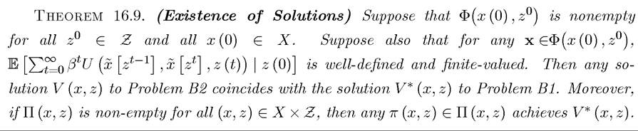
Notice that this theorem already imposes stronger requirements than Assumption 16.1 and hence there is no need to refer to Assumption 16.1.
Theorem 16.11. (Concavity of Value Functions) Suppose the hypotheses in Theorem 16.9 are satisfied and Assumptions 16.2* and 16.3* hold.
Then the unique function V that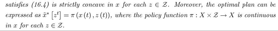
Theorem 16.12. (Monotonicity of Value Functions) Suppose the hypotheses in Theorem 16.9 are satisfied and Assumptions 16.2* and 16.4* hold. Then the unique value function V : X ? Z → R that satisfies (16.4) is strictly increasing in x for each z ∈ Z.
Theorem 16.13. (Differentiability of Value Functions) Suppose the hypotheses in
Theorem 16.9 are satisfied and Assumptions 16.2*, 16.3* and 16.5* hold. Let π be the policy
Given the hypotheses of Theorem 16.9, the proofs of these theorems are not difficult, though they are long and require a little care. Somewhat more general versions of these theorems can be found in Stokey, Lucas and Prescott (1989, Chapter 9), who first develop the necessary measure theory and some of the theory of general Markov processes to state more rigorous and complete versions of these theorems.
16.5.