A Baseline Model of Schumpeterian Growth
14.1.1. Preferences and Technology. In this section, we present a tractable model of Schumpeterian growth. We choose the economy to be as similar to the baseline (lab equipment) expanding machine variety model as possible, both to emphasize the parallels in the mathematical structures between these models and to highlight the basic economic differences that come from the presence of competition between new innovations and existing inputs (or products).
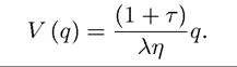
The economy is in continuous time and admits a representative household with the standard CRRA preferences, (13.1), as in the previous chapter. Population is constant at L and labor is supplied inelastically. The resource constraint at time t again takes the form where C (t) is consumption, X (t) is aggregate spending on machines, and Z (t) is total expenditure on R&D at time t.
 We again assume that there is a continuum of machines used in the production of a unique final good. Since there will be no expansion of inputs/machine variety, we normalize the measure of inputs to 1, and denote each machine line by ν ∈ [0,1]. The engine of economic growth here will be process innovations that lead to quality improvement. Let us first specify how the qualities of different machine lines change over time. Let q (ν, t) be the quality of machine line ν at time t. We assume the following “quality ladder” for each machine type:

where λ > 1 and n (ν, t) denotes the number of innovations on this machine line between time O and time t. This specification implies that there is a ladder of quality for each machine type, and each innovation takes the machine quality up by one rung in this ladder.
These rungs are proportionally equi-distant, so that each improvement leads to a proportional increase in quality by an amount λ > 1. Growth will be the result of these quality improvements.The production function of the final good is similar to that in the previous chapter, except that now the quality of the machines matters for productivity. We write the aggregate production function of the economy as follows:
where x(ν, t | q) is the quantity of the machine of type ν of quality q used in the production process. As in the previous chapter, this production function can be written as 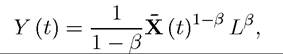 where
where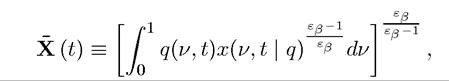
with which again emphasizes the continuity with the Dixit-Stiglitz model of Chap
ter 12.
An implicit assumption in (14.3) is that at any point in time only one quality of any machine is used. This is without loss of any generality, since in equilibrium only the highest- quality machines of each type will be used. This production function already indicates the source of creative destruction in this class on models: when a higher-quality machine is invented it will replace (“destroy”) the previous vintage of machines.
We next specify the technology for producing machines of different qualities and the innovation possibilities frontier of this economy. First, new machine vintages are invented by R&D. The R&D process is cumulative, in the sense that new R&D builds on an existing machine type. For example, consider the machine line ν that has quality q (ν, t) at time t. R&D on this machine line will attempt to improve over this quality. If a firm spends Z (ν, t) units of the final good for research on this machine line, then it generates a flow rate ηZ (ν, t) /q (ν, t) of innovation.
The innovation advances the knowhow on the production of this machine to the new rung of the quality ladder, thus creates a machine of type ν with quality λq (ν,t). Note that one unit of R&D spending is proportionately less effective when applied to a more advanced machine. This is intuitive, since we expect research on more advanced machines to be more difficult. It is also convenient from a mathematical point of view, since the benefit of research is also increasing with the quality of the machine (in particular, the quality improvements are proportional, with an innovation increasing quality from q (ν, t) to λq (ν, t)). Note that the costs of R&D are identical for the current incumbent and new firms (see Exercise 14.5 for alternative formulations). We assume that there is free entry into research, thus any firm or individual can undertake this type of research on any of the machine lines.As in the expanding varieties models of the previous chapter, the firm that makes an innovation has a perpetual patent on the new machine has invented. However, note that 507
the patent system does not preclude other firms undertaking research based on the product invented by this firm. We will discuss below how different patenting arrangements might affect incentives in this model.
Once a particular machine of quality q (ν, t) has been invented, any quantity of this machine can be produced at the marginal cost ψq (ν, t). Once again, the fact that the marginal cost is proportional to the quality of the machine is natural, since producing higher-quality machines should be more expensive.
One noteworthy issue here concerns the identity of the firm that will undertake R&D and innovation. In the expanding varieties model, this was irrelevant, since machines could not be improved upon, so there was only R&D for new machines, and who undertook the R&D was not important. Here, in contrast, existing machines can be (and are) improved, and this is the source of economic growth.
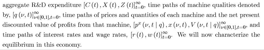
We have already seen in Chapter 12 that if the cost of R&D are identical for incumbents and new firms, Arrow’s replacement effect will imply that it will be the new entrants that undertake the R&D. The same applies in this model. The incumbent has weaker incentives to innovate, since it would be replacing its own machine, and thus destroying the profits that it is already making. In contrast, a new entrant does not have this replacement calculation in mind. As a result, with the same technology of innovation, it will always be the entrants that undertake the R&D investments in this model (see Exercise 14.1). This is an attractive implication, since it creates a real sense of creative destruction or churning. Of course in practice we observe established and leading firms undertaking innovations. This might be because the technology of innovation differs between incumbents and new potential entrants, or there is only a limited number of new entrants as in the model studied in Section 14.4 below (though in the current model this will not be sufficient, see Exercise 14.1).14.1.2. Equilibrium. An allocation in this economy is similar to that in the previous chapter. It consists of time paths of consumption levels, aggregate spending on machines, and
Let us start with the aggregate production function for the final good producers. A similar analysis to that in the previous chapter implies that the demand for machines is given by

where px (ν, t | q) refers to the price of machine type ν of quality q (ν, t) at time t. This expression stands for px (ν,t | q (ν, t)), but there should be no confusion in this notation since it is clear that q here refers to q (ν, t), and we will use this notation for other variables as well.
The price px (ν, t | q) will be determined by the profit-maximization of the monopolist holding the patent for machine of type ν of quality q (ν, t). Note that the demand from the final good sector for machines in (14.4) is iso-elastic as in the previous chapter, so the unconstrained monopoly price is again a constant markup over marginal cost. However, contrary to the situation in the previous chapter, there is now competition between firms that have access to different vintages of the machine. This implies that, as in our discussion in Chapter 12, we need to consider two regimes, one in which the innovation is “drastic” so that each firm can charge the unconstrained monopoly price, and the other one in which limit prices have to be used. Which regime we are in does not make any difference to the mathematical structure or to the substantive implications of the model. Nevertheless, we have to choose one of these two alternatives for consistency. Here we assume that the quality gap between a new machine and the machine that it replaces, λ, is sufficiently large, in particular, satisfies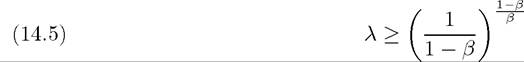
so that we are in the drastic innovations regime (see Exercise 14.7 for the derivation of this condition and Exercise 14.8 for the structure of the equilibrium under the alternative assumption). Let us also normalize ψ ? 1 — β as in the previous chapter, which implies that the profit-maximizing monopoly price is

Combining this with (14.4) implies that

Consequently, the flow profits of a firm with the monopoly rights on the machine of quality q(v,t) can be computed as:
This only differs from the flow profits in the previous chapter because of the presence of the quality term, q (ν,t).
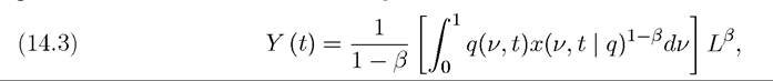
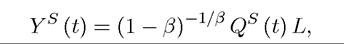
Next, substituting (14.7) into (14.3), we obtain that total output is given by
where
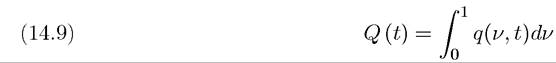
is the average total quality of machines. This expression closely parallels the derived production function (13.12) in the previous chapter, except that instead of the number of machine varieties, N (t), labor productivity is determined by the average quality of the machines, Q (t). This expression also clarifies the reasoning for the particular functional form assumptions above. In particular, the reader can verify that it is the linearity of the aggregate production function of the final good, (14.3) in the quality of machines that makes labor productivity depend on average qualities. With alternative assumptions, a similar expression to (14.8) would still obtain, but with a more complicated aggregator of machine qualities than the simple average (see, for example, Section 14.4). As a byproduct, we also obtain that aggregate spending on machines is

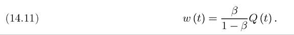
Similar to the previous chapter, labor, which is only used in the final good sector, receives an equilibrium wage rate of
We next specify the value function for the monopolist of variety ν of quality q (ν, t) at time t. As in the previous two chapters, despite the fact that each firm generates a stochastic stream of revenues, the presence of many firms with independent risks implies that each should maximize expected profits. The net present value of expected profits can be written in the Hamilton-Jacobi-Bellman form as follows

where z(ν, t | q) is the rate at which new innovations occur in sector ν at time t, while π(ν, t | q) is the flow of profits. This value function is somewhat different from the ones in the previous chapter (e.g., (13.8)), because of the last term on the right-hand side, which captures the essence of Schumpeterian growth. When a new innovation occurs, the existing monopolist loses its monopoly position and is replaced by the producer of the higher-quality machine. From then on, it receives zero profits, and thus has zero value. In writing this equation, we have made use of the fact that because of Arrow’s replacement effect, it is an entrant that is undertaking the innovation, thus z(ν, t | q) corresponds to the flow rate at which the incumbent will be replaced by a new entrant.
Free entry again implies that we must have

In other words, the value of spending one unit of the final good should not be strictly positive. Recall that one unit of the final good spent on R&D for a machine of quality λ-1q has a flow rate of success equal to η/ (λ-1q), and in this case, it generates a new machine of quality 510
q, which will have a net present value gain of V(ν,t | q). If there is positive R&D, i.e., Z (ν,t | q) > 0, then the free entry condition must hold as equality.
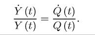
Note also that even though the quality of individual machines, the q (ν, t)'s, are stochastic (and depend on success in R&D), as long as R&D expenditures, the Z (ν,t | q)'s, are nonstochastic, average quality Q (t), and thus total output, Y (t), and total spending on machines, X (t), will be nonstochastic. This feature will significantly simplify notation and the analysis of this economy.
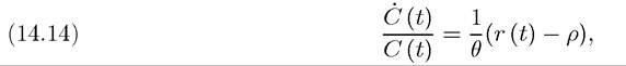
Consumer maximization again implies the familiar Euler equation,
and the transversality condition takes the form
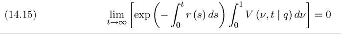
for all q. This transversality condition follows because now the total value of corporate assets is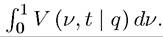 Even though the evolution of the quality of each machine line is
stochastic, the value of a machine of type ν of quality q at time t, V (ν,t | q), is nonstochastic. Either q is not the highest quality in this machine line, in which case V (ν, t | q) is equal to 0, or alternatively, it is given by (14.12).
These equations complete the description of the environment. An equilibrium can then be
We will first focus on an equilibrium path with balance growth, i.e., on the the balanced growth path (BGP), where output and consumption grow at constant rates.
14.1.3. Balanced Growth Path. In the balanced growth path (BGP), consumption grows at the constant rate With familiar arguments, this must be the same rate as output growth, g*. Moreover, from (14.14), the interest rate must be constant, i.e., r (t) = r* for all t.
If there is positive growth in this BGP equilibrium, then there must be research at least in some sectors. Since both profits and R&D costs are proportional to quality, whenever the free entry condition (14.13) holds as equality for one machine type, it will hold as equality 511
for all of them. This, in turn, implies that
(14.16)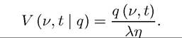
Moreover, if it holds between t and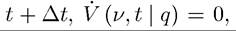 because the right-hand side of
equation (14.16) is constant over time—q (ν,t) refers to the quality of the machine supplied by the incumbent, which does not change. Since R&D for each machine type has the same productivity, this implies that z (ν, t) must also be the same for all machine types, thus equal to some z (t). Moreover, in BGP, this rate will be constant and we will denote it by z*. Then (14.12) implies (
Notice the difference between this value function and those in the previous chapter: instead of the discount rate r*, the effective discount rate is r* + z*, since incumbent monopolists understand that competitive innovations will replace them.
Combining this equation with (14.16), we obtain

Moreover, from the fact that

To solve for the BGP equilibrium, we need a final equation relating the BGP growth rate of the economy, g*, to z*. From (14.8)
Next, note that, by definition, in an interval of time ∆t, there will be z (t) ∆t sectors that experience one innovation, and this will increase their productivity by λ. The measure of sectors experiencing more than one innovation within this time interval is o (∆t)—i.e., it is second-order in ∆t, so that as ∆t → 0, o(∆t)∕∆t → 0. Therefore, we have

Now subtracting Q (t) from both sides, dividing by ∆t and taking the limit as ∆t → 0, we obtain
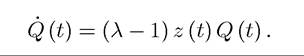
Therefore,

512
Now combining (14.18)-(14.20), we obtain the BGP growth rate of output and consumption
as:
id="Picutre 1690" class="lazyload" data-src="/files/uch_group77/uch_pgroup317/uch_uch7364/image/image1688.jpg">
This establishes the following proposition
PROPOSITION 14.1. Consider the model of Schumpeterian growth described above. Suppose that

Then, there exists a unique balanced growth path in which average quality of machines, output and consumption grow at rate g* given by (14.21). The rate of innovation is g* / (λ — 1).
Proof. Most of the proof is given in the preceding analysis. In Exercise 14.3 you are asked to check that the BGP equilibrium is unique and satisfies the transversality condition.
?
The above analysis illustrates that the mathematical structure of the model is quite similar to those analyzed in the previous chapter. Nevertheless, the feature of creative destruction, the process of incumbent monopolists being replaced by new entrants, is new and provides a very different interpretation of the growth process. We will return to some of the applications of creative destruction below.
Before doing this, we can also analyze transitional dynamics in this economy. Similar arguments to those used in the previous chapter establish the following result:
PROPOSITION 14.2. In the model of Schumpeterian growth described above, starting with any average quality of machines Q (0) > 0, there are no transitional dynamics and the equilibrium path always involves constant growth at the rate g* given by (14.21).
Proof. See Exercise 14.4. ?
A notable feature of the model, which is again related to the functional form of the aggregate production function (14.3), is that only the average quality of machines, Q (t), matters for the allocation of resources. Moreover, the incentives to undertake research are identical for two machine types ν and with different quality levels q (ν, t) and
 thus there is no incentive to undertake different R&D investments for more and less advanced machines. This is again a feature of the functional forms chosen here, and Exercise 14.13 shows that in different circumstances this result may not apply. Nevertheless, the specification chosen in this section is appealing, since it implies that research will be directed at a broad range of machines rather than a specific subset of the available types of machines.
14.1.4. Pareto Optimality. This equilibrium, like that of the endogenous technology model with expanding varieties, is typically Pareto suboptimal. The first reason for this is the appropriability effect, which results because monopolists are not able to capture the entire social gain created by an innovation. However, Schumpeterian growth also introduces the business stealing effect discussed in Chapter 12. Consequently, the equilibrium rate of innovation and growth can now be too high or too low. We now investigate this question.
We proceed as in the previous chapter, first deriving quantities of machines that will be used in the final good sector by the social planner. In the social planner’s allocation there is no markup on machines, thus we have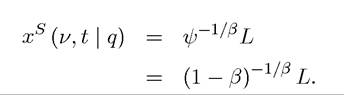
Substituting this into (14.3), we obtain
where again the superscript S refers to the social planner’s allocation. The net output that can be distributed between consumption and research expenditure is
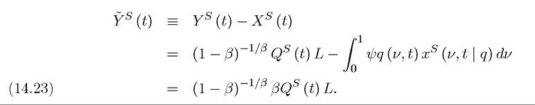
Moreover, given the specification of the innovation possibilities frontier above, the social planner can improve the aggregate technology as follows:
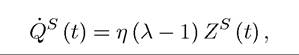
since an R&D spending of Zs (t) will lead to discoveries of better vintages at the flow rate of η and each of these vintages increases average quality of machines by a proportional amount λ - 1.
Now, given this equation, the maximization problem of the social planner can be written as
subject to

where the constraint equation uses net output, (14.23), and the resource constraint, (14.1). In this problem, Qs (t) is the state variable, and Cs (t) is the control variable. It can be verified that this problem satisfies all the assumptions of Theorems 7.9 and 7.12, so a solution that 514
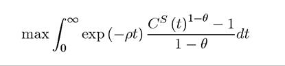
satisfies the necessary conditions in Theorem 7.9 will give the unique optimal growth path. To characterize this solution, let us set up the current-value Hamiltonian as

The necessary conditions for a maximum are
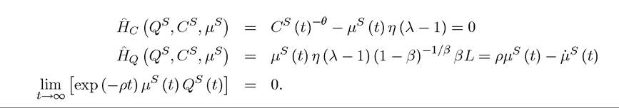
Moreover, it is straightforward to verify that the current-value Hamiltonian is concave in C and Q, so any solution to these necessary conditions is an optimal plan. Combining these conditions, we obtain the following growth rate for consumption in the social planner’s allocation (see Exercise 14.6):
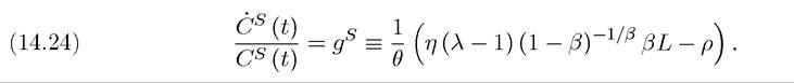
Clearly, total output and average quality will also grow at the rate gs in this allocation.
Comparing gs to g* in (14.21), we can see that either could be greater. In particular, when λ is very large, gs > g*, and there is insufficient growth in the equilibrium. We can see this as follows: as In contrast, to obtain an example
in which there is excessive growth in the equilibrium, suppose that θ = 1, β = 0.9, λ = 1.3, η = 1, L = 1 and ρ = 0.38. In this case, it can be verified that gs ≈ 0, while g* ≈ 0.18 > gs.[XXIV]
This illustrates the counteracting influences of the appropriability and business stealing effects discussed above. The following proposition summarizes this result:
PROPOSITION 14.3. In the model of Schumpeterian growth described above, the decentralized equilibrium is generally Pareto suboptimal, and may have a higher or lower rate of innovation and growth than the Pareto optimal allocation.
It is also straightforward to verify that as in the models of the previous section, there is a scale effect, and thus population growth would lead to an exploding growth path. Exercise 14.10 asks you to construct an endogenous growth model of Schumpeterian growth without scale effects.
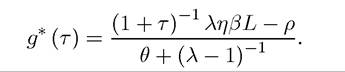
14.1.5. Policy in the Model of Schumpeterian Growth. We now use the Schumpeterian growth model to analyze the effects of policy on economic growth. As in the model of the previous few chapters, anti-trust policy, patent policy and taxation will affect the equilibrium growth rate. For example, two economies that tax corporate incomes at different rates, say τ and τ0, will grow at different rates.
There is a sense in which the current model is much more appropriate for conducting policy analysis than the expanding varieties models, however. In those models, there was no reason for any agent in the economy to support distortionary taxes (which reduce the growth rate).* [XXV] In contrast, the fact that growth takes place through creative destruction here implies that there is a natural conflict of interest, and certain types of policies may have a constituency. To illustrate this point, which will be discussed in greater detail in Part 8 of the book, suppose that there is a tax τ imposed on R&D spending. This has no effect on the profits of existing monopolists, and only influences their net present discounted value via replacement. Since taxes on R&D will discourage R&D, there will be replacement at a slower rate, i.e., z* will fall. This increases the steady-state value of all monopolists given by (14.17). In particular, denoting the value of a monopolist with a machine of quality q by where the equilibrium interest rate and the replacement rate have been written as functions of τ. With the tax rate on R&D, the free entry condition, (14.13) becomes This equation shows that V (q) is clearly increasing in the tax rate on R&D, τ. Combining the previous two equations, we see that in response to a positive rate of taxation, r* (τ) + z* (τ) must adjust downward, so that the value of current monopolists increases (consistent with the previous equation). Intuitively, when the costs of R&D are raised because of tax policy, the value of a successful innovation, V (q), must increase to satisfy the free entry condition. This can only happen through a decline the effective discount rate r* (τ) + z* (τ). A lower effective discount rate, in turn, is achieved by a decline in the equilibrium growth rate of the economy, which now takes the form It is straightforward to verify that this growth rate is strictly decreasing in τ. Nevertheless, as the previous expression shows, incumbent monopolists would be in favor of increasing τ in order to shield themselves from the competition of new entrants. Essentially, in this 2 model, slowing down the process of creative destruction is beneficial for incumbents, creating a rationale for growth-retarding policies to emerge in equilibrium. Therefore, an important advantage of models of Schumpeterian growth is that they start providing us clues about why some societies may adopt policies that reduce the growth rate. Since taxing R&D by new entrants benefits incumbent monopolists, when incumbents are sufficiently powerful politically, such distortionary taxes can emerge in the political economy equilibrium, even though they are not in the interest of the society at large. 14.2.