A One-Sector Schumpeterian Growth Model
The model of Schumpeterian growth presented in the previous section was designed to maximize the parallels between this class of models and those based on expanding varieties. In this section, we discuss a model more closely related to the original Aghion and Howitt (1992) setup, which is simpler in some ways and more complicated in others.
Relative to the model presented in the previous section, it has two major differences. First, there is only one sector experiencing quality improvements rather than a continuum of machine types. Second, the innovation possibilities frontier uses a scarce factor, labor, as in the model of knowledge spillovers in Section 13.2 of the previous chapter. Since there are many parallels between this model and those we have studied so far, we will provide only a brief exposition of this model.14.2.1. The Basic Aghion-Howitt Model. The consumer side is the same as before, with the only difference that we now assume consumers are risk neutral, so that the interest rate is determined as
at all points in time. Population is again constant at a level L and all individuals supply labor inelastically. The aggregate production function of the unique final good is now given by

where q (t) is the quality of the unique machine used in production and is written in the labor-augmenting form for simplicity; x (t | q) is the quantity of this machine used at time t; and Le (t) denotes the amount labor used in production at time t, which is less than L, since Lr (t) workers will be employed in the R&D sector. Market clearing requires that
Once invented, a machine of quality q (t) can be produced at the constant marginal cost ψ in terms of final goods.
We again normalize ψ ? 1 — β. The innovation possibilities frontier now involves labor being used for R&D. In particular, each worker employed in the R&D sector 517generates a flow rate η of a new machine. When the current machine used in production has quality q (t), the new machine has quality λq (t).
Let us once again assume that (14.5) above is satisfied, so that the monopolist can charge the unconstrained monopoly price. Then, an analysis similar to that in the previous section immediately implies that the demand for the leading-edge machine of quality q is given by  where again px (ν, t) denotes the price of the machine of quality q. The monopoly price for the highest quality machine is:[26]
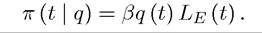
for all q and t. Consequently, the demand for the machine of quality q at time t is given by  and monopoly profits are
We can also write aggregate output as
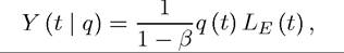
where we again condition on the quality of the machine available at the time, q. This also implies that the equilibrium wage, determined from the final good sector, is given by
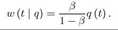
When there is no need to emphasize time dependence, we will write this wage rate as a function of machine quality, i.e., as w (q).
Let us now focus on a “steady-state equilibrium” in which the flow rate of innovation is constant and equal to z*. Steady state here is an quotation marks since, even though the flow rate of innovation is constant, consumption and output growth will not be constant because of the stochastic nature of innovation (and this is the reason why we do not use the term “balanced growth path” in this context).
This implies that a constant number (and thus a constant fraction) of workers, LR, must be working in research. Since the interest rate is equal to r* = ρ, this implies that the steady-state value of a monopolist with a machine of quality q is given by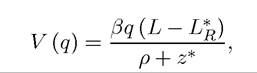
where we have used the fact that in steady state total employment in the final good sector is equal to To simplify the notation, we also wrote V as a function of q
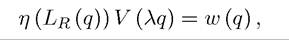
only rather than a function of both q and time. Free entry requires that when the current machine quality is q, the wage paid to one more R&D worker, w (q), must be equal to the flow benefits, ηV (λq), thus
Flow benefits from R&D are equal to ηV (λq), since, when current machine quality is q, one more worker in R&D leads to the discovery of a new machine of quality λq at the flow rate η. In addition, given the R&D technology, we must hav Combining the last four
equations we obtain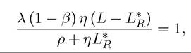
which uniquely determines the steady-state number of workers in research as
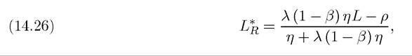
as long as this expression is positive.
Contrary to the model in the previous section, however, this does not imply that output grows at a constant rate. Since there is only one sector undergoing technological change and this sector experiences growth only at finite intervals, the growth rate of the economy will have an uneven nature; in particular, it can be verified that the economy will have constant output for an interval of time (of average length see Exercise 14.15) and then will have a burst of growth when a new machine is invented.
The results of this analysis are summarized in the next proposition.
PROPOSITION 14.4. Consider the one-sector Schumpeterian growth model presented in this section and suppose that

Then there exists a unique steady-state equilibrium in which L*r workers work in the research sector, where L*r is given in equation (14.26). The economy has an average growth rate of 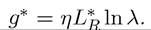 Equilibrium growth is “uneven,” in the sense that the economy has constant output for a while and then grows by a discrete amount when an innovation takes place.
Proof. Much of the proof is provided by the preceding analysis. Exercise 14.16 asks you to verify that the average growth is given by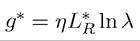 and that (14.27) is necessary for
the above described equilibrium to exist and to satisfy the transversality condition. ?
Therefore, this analysis shows that the basic insights of the one-sector Schumpeterian model, as originally developed by Aghion and Howitt (1992), are very similar to the baseline model of Schumpeterian growth presented in the previous section. The main difference is that growth has an uneven flavor in the one-sector model, because it is driven by infrequent bursts of innovation, preceded and followed by periods of no growth.
14.2.2. Uneven Growth and Endogenous Cycles*. The analysis in the previous subsection showed how the basic one-sector Schumpeterian growth leads to an uneven pattern of economic growth.
This is driven by the discrete nature of innovations in continuous time. There is another source of uneven growth in this basic model, which is more closely related to the process of creative destruction. The nature of Schumpeterian growth implies that future growth reduces the value of current innovations, because it causes more rapid replacement of existing technologies. This effect did not play a role in our analysis so far, because in the model with a continuum of sectors, growth takes a smooth form and as Proposition 14.2 showed, there is a unique equilibrium path with no transitional dynamics. The one-sector growth model analyzed in this section allows these effects to manifest themselves. To show the potential for these creative destruction effects, we now construct a variant of the model which exhibits endogenous growth cycles. Throughout, we focus on an equilibrium path with such a cycle.The only difference is that we now assume that the technology of R&D implies that Lr workers in research leads to innovation at the rate
where η (∙) is a strictly decreasing function, representing an externality in the research process. When more firms try to discover the next generation of technology, there will be more crowding-out in the research process, making it less likely for each of them to innovate. Each firm ignores its effect on the aggregate rate of innovation, thus takes η (Lr) as given (this assumption is not important as shown by Exercise 14.21). Consequently, when the current machine quality is q, the free entry condition takes the form
where Lr (q) is the number of workers employed in research when the current machine quality is q.
Let us now look for an equilibrium with the following cyclical property: the rate of innovation differs when the innovation in question is an odd-numbered innovation versus an 520
even-numbered innovation (say with the number of innovations counted starting from some arbitrary date t = 0).
This type of equilibrium is possible when all agents in the economy expect there to be such an equilibrium (i.e., it is a “self-fulfilling” equilibrium). Denote the number of workers in R&D for odd and even-numbered innovations by Then,
Then, following the analysis in the previous subsection, in any equilibrium with a cyclical pattern the values of odd and even-numbered innovations (with a machine of quality q) can be written as (see Exercise 14.19):

and the free entry conditions take the form

where w (q) is the equilibrium wage with technology of quality q. The reason why multiplies the value for an even-numbered innovation is because LR researchers are employed for innovation today, when the current technology is odd-numbered, but the innovation that this research will produce will be even-numbered and thus will have value V2 (λq). Therefore, we have the following two equilibrium conditions:
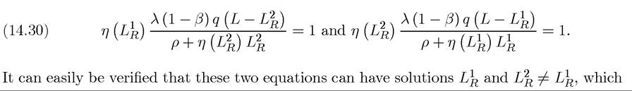
would correspond to the possibility of a two-period endogenous cycle (see Exercise 14.20).
14.2.3. Labor Market Implications of Creative Destruction. Another important implication of creative destruction is related to the fact that growth destroys existing productive units. So far this only led to the destruction of the monopoly rents of incumbent producers, without any loss of employment. In more realistic economies, creative destruction may dislocate previously employed workers and these workers may experience some unemployment before finding a new job. How creative destruction may lead to unemployment is discussed in Exercise 14.18.
A final implication of creative destruction that is worth noting relates to the destruction of firm-specific skills. It may be efficient for workers to accumulate human capital that is specific to their employers. Creative destruction implies that productive units may have shorter horizons in an economy with rapid economic growth. An important consequence of this might be that in rapidly growing economies, workers (and sometimes firms) may be less willing to make a range of specific human capital and other investments.
14.3.