Innovation by Incumbents and Entrants and Sources of Productivity Growth

A key aspect of the growth process is the interplay between innovations and productivity improvements by existing firms on the one hand and entry by more productive, new firms on the other.

14.3.1. Model. The economy is again in continuous time and admits a representative household with the standard CRRA preferences, as in (13.1) in the previous chapter. Popu­lation is constant at L and labor is supplied inelastically. The resource constraint at time t takes the usual form

(14.31) C (t)+ X (t) + Z (t) ≤ Y (t),

where C (t) is consumption, X (t) is aggregate spending on machines, and Z (t) is total expenditure on R&D at time t.

The production function of the unique final good is given by:

where x(ν, t | q) is the quantity of the machine of type ν of quality q used in the production process and the measure of machines is again normalized to 1. This production is very similar to (14.3) used above, except that the quality of machines comes in with an exponent β. This has no effects on any of the results concerning growth, but will imply that firms

with different productivity levels will have different levels of sales (see Exercise 14.26). It will therefore enable us to make predictions about the size distribution of firms as well.

The engine of economic growth is again quality improvements, but these will be driven by two types of innovations:

(1) Innovation by incumbents

(2) Creative destruction by entrants.

Let q (ν, t) be the quality of machine line ν at time t. We assume the following “quality ladder” for each machine type:

where λ > 1 and n (ν, t) denotes the number of incremental innovations on this machine line between time s ≤ t and time t, where time s is the date at which this particular type of technology was first invented and q (ν, s) refers to its quality at that point. The incumbent has a fully enforced patent on the machines that it has developed (though this patent does not prevent entrants leapfrogging the incumbent’s machine quality). We assume that at time t = 0, each machine line starts with some quality q (ν, 0) > 0 owned by an incumbent with fully enforce patent on this initial machine quality. Incremental innovations can only be performed by the incumbent producer. So we can think of those as “tinkering” innovations that improve the quality of the machine. The assumption that incumbents have access to a technology to create incremental innovations is consistent with case study evidence on industry level innovation (e.g., Freemen, 1982, or Sherer, 1984).

More specifically, if the current incumbent spends an amount z (ν, t) q (ν, t) of the final good for this type of innovation activity on a machine of current quality q (ν,t), it has a flow rate of innovation equal to φz (ν, t) for φ > 0 (more formally, this implies that for any interval ∆t > 0, the probability of one incremental innovation is φz (ν, t) ∆t and the probability of more than one incremental innovation is o (∆t) (with o (∆t) /∆t → 0 as ∆t → 0). Recall that such an innovation results in an improvement in quality and the resulting new machine will be of quality λq (ν, t).

Alternatively, a new firm (entrant) can undertake R&D to innovate over the existing machines in machine line ν at time t. If the current quality of machine is q (ν, t), then by spending one unit of the final good, this new firm has a flow rate of innovation equal to Incumbents can also be allowed to have access to the same technology for radical innovation as the entrants. However, the Arrow replacement effect then immediately implies that incum­bents would never use this technology (since entrants will be making zero profits from this technology, the profits of incumbents would be negative; see Exercise 14.22). Incumbents will 523

still find it profitable to use the technology for incremental innovations, which is not available to entrants.

The presence of the strictly decreasing function η, which was also used in Section 14.2, captures the fact that when many firms are undertaking R&D to replace the same machine line, they are likely to try similar ideas, thus there will be some amount of “external” di­minishing returns (new entrants will be “fishing out of the same pond”). Since each entrant attempting R&D on this line is potentially small, they will all takeas given.

Throughout I assume that zη (z) is strictly increasing in z so that greater aggregate R&D towards a particular machine line increases the overall probability of discovering a superior machine. I also suppose that η (z) satisfies the following Inada-type assumptions:

An innovation by an entrant leads to a new machine of quality κq (ν,t), where ê > λ. Therefore, innovation by entrants are more “radical” than those of incumbents. Existing empirical evidence from studies of innovation support the notion that innovations by new entrants are more significant or radical than those of incumbents (though it may take a while for the successful entrants to realize the full productivity gains from these innovations; I am abstracting from this aspect). Importantly, whether the entrant was a previous incumbent on this specific machine line or whether it its currency an incumbent in some other machine line do not matter for its technology of innovation.

Once a particular machine of quality q (ν, t) has been invented, any quantity of this machine can be produced at the marginal cost ψ. I again normalize ψ ? 1 — β. This implies that the total amount of expenditure on the production of intermediate goods at time t is where x (ν,t) is the quantity of this machine used in final good production. Similarly, the total expenditure on R&D is

1739" class="lazyload" data-src="/files/uch_group77/uch_pgroup317/uch_uch7364/image/image1737.jpg">

where q (ν, t) refers to the highest quality of the machine of type ν at time t. Notice also that total R&D is the sum of R&D by incumbents and entrants (z (ν, t) and Z (ν, t) respectively).

An allocation in this economy consists of time paths of consumption levels, aggregate spending on machines, and aggregate R&D expendituretime paths

for R&D expenditure by incumbent and entrantstime paths of

prices and quantities of each machine and the net present discounted value of profits from that machine,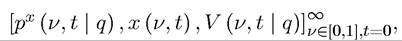and time paths of interest rates and

wage rates,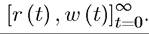An equilibrium is given by an allocation in which R&D decisions

by entrants maximize their net present discounted value, pricing, quantity and R&D decisions 524

by incumbents maximize their net present discounted value, consumers choose the path of consumption optimally, and the labor market clears.

Let us start with the aggregate production function for the final good producers. Profit­maximization by the final good sector implies the demand for machines of highest-quality is given by a slight variant of equation (14.4) in Section 14.1:

where p^x (ν, t | q) refers to the price of machine type ν of quality q (ν, t) at time t. Since the demand from the final good sector for machines in (14.36) is iso-elastic, the unconstrained monopoly price will given by the usual formula as a constant markup over marginal cost. In this context, I introduced the analogue of condition (14.5) above,

which ensures that new entrants can charge the unconstrained monopoly price. By implica­tion, incumbents that make further innovations can also charge the unconstrained monopoly price.

14.3.2. Equilibrium. Since the demand for machines in (14.36) is iso-elastic and ψ = 1 — β, the profit-maximizing monopoly price is

Combining this with (14.36) implies that

Consequently, the flow profits of a firm with the monopoly rights on the machine of quality q can be computed as:

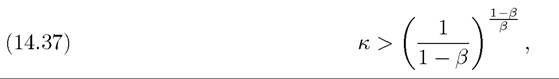
Next, substituting (14.39) into (14.32), we obtain that total output is given by an expression identical to (14.8) above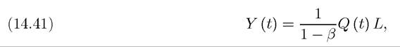

with average quality of machines Q (t) given as in (14.9) in Section 14.1.

As a byproduct, we also obtain that aggregate spending on machines is

Moreover, since the labor market is competitive, the wage rate at any point in time is given by (14.11) as before.

To characterize the full equilibrium, we need to determine R&D effort levels by incum­bents and entrants. To do this, let us write the net present value of a monopolist with the 525

highest quality of machine q at time t in machine line ν. This value satisfies the standard Hamilton-Jacobi-Bellman equation:

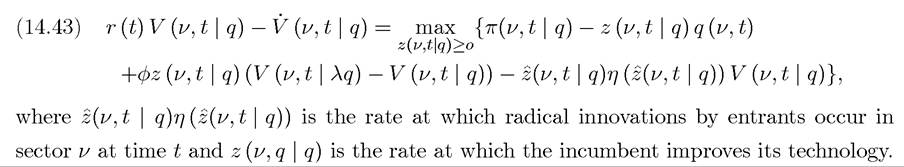
The first term in (14.43), π(ν,t | q), is the flow of profits given by (14.40), while the second term is the expenditure of the incumbent for improving the quality of its product. The second line includes changes in the value of the incumbent due to innovation either by itself (at the rate φz (ν,t | q), the quality of its product increases from q to λq) or by an entrant (at the rate Z(ν, t | q)η (Z(ν, t | q)), the incumbent is replaced and receives zero value from then on).^[28] The value function is written with a maximum on the right hand side, since z (ν,t | q) is a choice variable for the incumbent.

Free entry by entrants implies that we must have a free entry condition similar to (14.13) in Section 14.1:

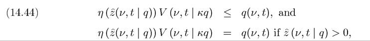
which takes into account that by spending an amount q(ν,t), the entrant generates a flow rate of innovation of η (Z), and if this innovation is successful, the entrant will end up with a product of quality κq, thus earning the value

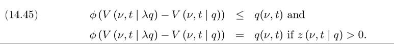
In addition, the incumbent’s choice of R&D effort implies a similar complementary slack­ness condition

Finally, consumer maximization implies the familiar Euler equation and the transversality condition given by (14.14) and (14.15) as before.

In light of this analysis, an equilibrium can be more succinctly defined as time path of

As usual, I define a BGP (balanced growth path) as an equilibrium path in which innova­tion, output and consumption growth a constant rate. Notice that in BGP, aggregates grow at the constant rate, but there will be firm deaths and births, and the firm size distribution may also change.

The requirement that consumption grows at a constant rate in the BGP implies that for all q, it is not necessarily true that z (q) = z for all q. In fact, as we will see the equilibrium only pins down the average R&D intensity of incumbents.

Let us first look for an “interior” BGP equilibrium (we will verify below that such an interior BGP exists and is the unique equilibrium). This implies that incumbents undertake research, thus

Given the linearity of V in q, this implies the following convenient equation for the value of a firm with a machine of quality q :

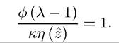
Moreover, from the free entry condition (again holding as equality since the BGP is interior) we have that

Moreover, from the free entry condition (again holding as equality from the fact that the equilibrium is interior):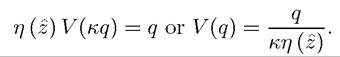

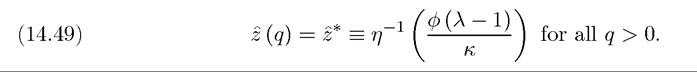
Combining this expression with (14.46) and (14.47), we obtain

This implies that the BGP R&D level by entrants Z* is implicitly defined by

Next, combining this with (14.48), we obtain the BGP interest rate as

527

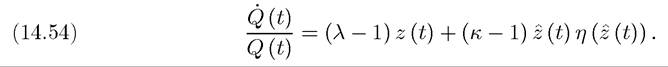
From (14.14), the growth rate of consumption and output is therefore given by

id="Picutre 1764" class="lazyload" data-src="/files/uch_group77/uch_pgroup317/uch_uch7364/image/image1762.jpg">

Equation (14.51) already has some interesting implications. In particular, it determines the relationship between the rate of innovation by entrantsand the BGP growth rate g*. In standard Schumpeterian models, this relationship is positive. In contrast, here we have the following immediate result:

Proposition 14.5. There is a negative relationship between Z* and g*.

Equation (14.51), together with (14.49), determines the BGP growth rate of the economy, but does not specify how much of productivity growth is driven by creative destruction (innovation by entrants) and how much of it by productivity improvements by incumbents. To determine this, we repeat the same analysis as in Section 14.1. Recall, at this point, that z (ν,t | q) is not a function of ν, but could still depend on q. Consequently, we can obtain the law of motion of average quality, Q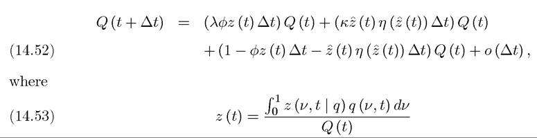(t), as

is the average R&D effort of incumbents that time t. Now subtracting Q (t) from both sides of (14.52), dividing by ∆t and taking the limit as ∆t → 0, we obtain

Therefore, an alternative expression for the growth rate of the economy, which decomposes growth into the component coming from incumbent firms (the first term) and that coming from new entrants (the second term) is given as

where z* is the average BGP R&D effort of incumbents. The fact that this average R&D effort is constant in BGP follows from the fact from (14.54) together with the fact that in BGP the growth rate of average quality is g* and the R&D effort by entrants on each machine line is Z*. While (14.51) pins down the BGP growth rate of output and consumption, equation (14.55) determines how much of it is driven by innovation by incumbents and how much of it by innovation by entrants. Moreover, we can also verify that this economy does not have any transitional dynamics (see the proof of Proposition 14.6). Therefore, if an equilibrium with growth exists, it will involve growth at the rate g*. To ensure that such an equilibrium exists, 528

we need to verify that R&D is profitable both for entrants and incumbents. The condition that the BGP interest rate, r*, given by (14.50), should be greater than the discount rate ρ is sufficient for there to be positive aggregate growth. In addition, this interest rate should not be so high that the transversality condition of the consumers is violated. Finally, we need to ensure that there is also innovation by incumbents. The following condition ensures all three of these requirements (see the proof of Proposition 14.6):

with z* given by (14.49).

In addition, our main interest is with how much of productivity growth and innovation are driven by incumbents and how much by new entrants. This can now be easily obtained from (14.51) and (14.55) as

where g* is given by (14.51) and z* by (14.49).

Another set of interesting implications of this model concern firm-size dynamics. The size of a firm can be measured by its sales, which is equal to

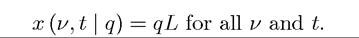
To determine the law of motion of firm sales and thus the firm-size dynamics, we need to know how incumbent R&D effort varies with q. To start with, let us suppose that in BGP this R&D effort is independent of q, so that z (ν,t | q) = z* for all q. From the analysis so far, it is clear that such an equilibrium will exist (for a justification of the focus on this 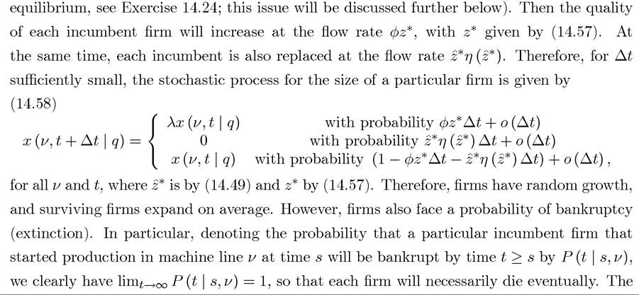implications of equation (14.58) for the the stationary firm size distribution is discussed in subsection 14.3.5 below.

The following proposition summarizes the main results of this section.

PROPOSITION 14.6. Consider the above-described economy starting with an initial condi­tion Q (0) > 0. Suppose that (14.33) and (14.56) are satisfied and focus on equilibrium in which all incumbents exert the same level of R&D effort. Then there exists a unique equilib­rium. In this equilibrium growth is always balanced, and technology, Q (t), aggregate output, Y (t), and aggregate consumption, C (t), grow at the rate g* as in (1f.51) withgiven by (14.49). Equilibrium growth is driven both by innovation by incumbents and by creative destruction by entrants. Any given firm expands on average as long as it survives, but is eventually replaced by a new entrant with probability one.

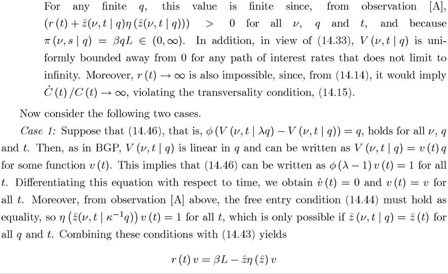
PROOF. First, note that in an interior BGP where φ (V (ν,t | λq) — V (ν,t | q)) = q, V must be linear in q, thus V (ν,t | q) = vq as used in the text. Given this observation, the characterization of the BGP follows from the argument preceding the proposition. In particular, z* is uniquely determined by (14.49) and (14.51) gives the unique BGP growth rate. To ensure that this is indeed an interior BGP, we need to check four conditions:

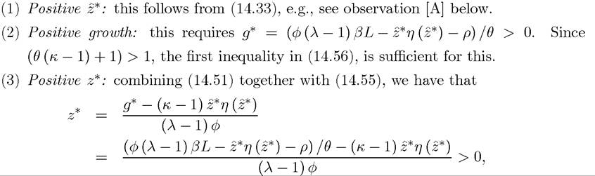
in view of the first inequality (14.56).

(4) The transversality condition: condition (14.15) should hold so that the maximization

problem of the representative household is well-defined. The condition r* > g* is necessary and sufficient to ensure (14.15). The second inequality in (14.56) ensures that this inequality holds.

Therefore, the BGP is interior and is uniquely defined.

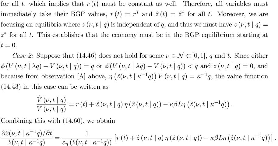
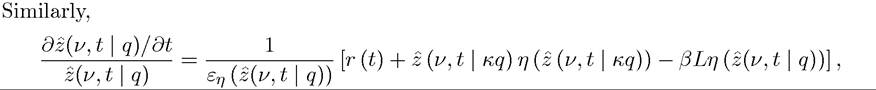
I next prove that the BGP also gives the unique dynamic equilibrium path. Let us start with two observations.

[A] Because of the Inada conditions, (14.33), the free entry condition (14.13) must hold as equality for all ν, t and q, so that

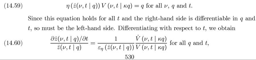
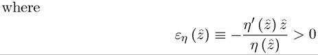
is the elasticity of the η function.

[B] The value of a firm with a machine of quality q at time t can be written as

and so on. It is then straightforward to see that the system of differential equations for

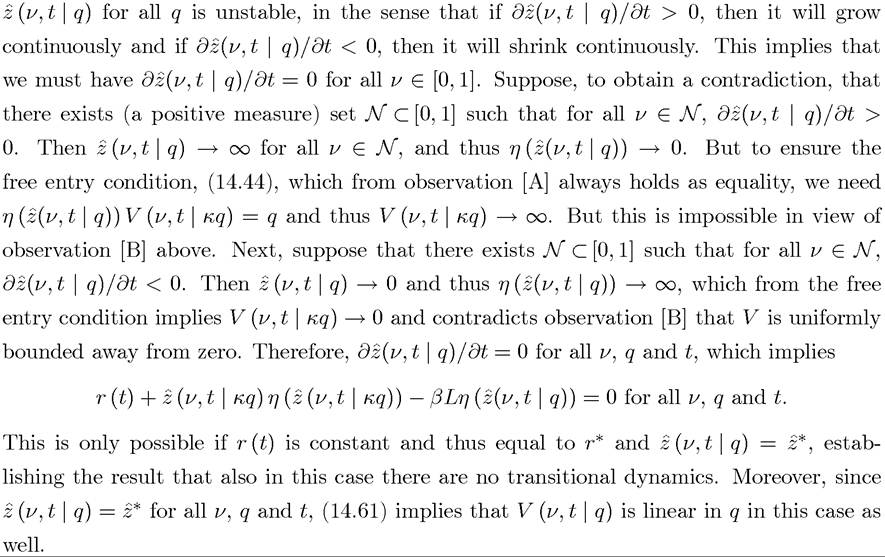
Finally, the result that surviving firms expand on average and that all firms die with probability 1 follows from equation (14.58). ?

Proposition 14.6 focuses on equilibria in which all incumbents exert the same R&D effort.

Exercise 14.25 shows that the same conclusions hold when we do not focus on such equilibria.

14.3.3. Some Numbers. I will now try to flesh out the implications of this model on the decomposition of productivity growth between incumbents and entrants. Although some of the parameters of the current model are difficult to pin down with our current knowledge of the technology of R&D, some simple back-of-the-envelope calculations are still informative. Let us choose the following standard numbers:

where the last number, the intertemporal elasticity of substitution, is pinned down by the choice of the other three numbers. The first three numbers refer to annual rates (implicitly defining ∆t = 1 as one year). We have much greater uncertainty concerning the remaining parameters. We can normalize φ = L = 1. For the rest, I will report a number of different possibilities. As a benchmark, As a benchmark, I take β = 2/3, which implies that two 532

thirds of national income accrues to labor and one third to profits. The requirement in (14.37) then implies that ê > 1.7. I also take the benchmark value of κ = 3, so that entry by new firms is sufficiently “radical” as suggested by some of the qualitative accounts of the innovation process (e.g., Freeman, 1982, Scherer, 1984). Innovation by incumbents is taken to be correspondingly smaller λ = 1.2. This implies that productivity gains from a radical innovation is about ten times that of a standard “incremental” innovation by incumbents (i.e., (κ — 1) / (λ — 1) = 10). I will then show how the results change when the magnitudes of radical and incremental innovations are varied. For the function η (z), I adopt the following frequently-used form: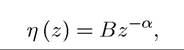

and choose the benchmark value of α = 0.5. The remaining two parameters, φ and B will be chosen to ensure g* = 0.02. I start with the benchmark value of φ = 0.4, but this value will need to be modified in some of the variations in order to satisfy condition (14.56) above or to ensure g* = 0.02. With these numbers, (14.49) implies

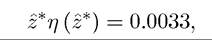
and

The value foralso implies that there is entry of a new firm (creative destruction) in each machine line on average once every 7.5 years (recall that r* = 0.05 as the annual interest rate so that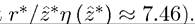Next, using (14.55), the contribution of productivity growth

by continuing firms is

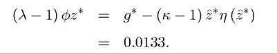
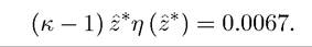
Therefore, in this benchmark parameterization, over two thirds of productivity growth comes from innovation by incumbents. Moreover, φz* = 0.0667, so that there are on average 1.2 incremental innovations per year by an incumbent in a particular machine line.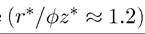

Using alternative values of the parameters κ, λ, β and α leads to broadly similar conclusions, though depending on the exact parameterization the contribution of entrants to productivity growth can be larger or smaller.

14.3.4. The Effects of Policy on Growth. Let us now use this model to analyze the effects of policies on equilibrium productivity growth and its decomposition between incumbents and entrants. Since the model has a Schumpeterian structure (with quality improvements as the engine of growth and creative destruction playing a major role), it may be conjectured that entry barriers (or taxes on potential entrance) will have negative effects on economic growth as in the baseline model we studied earlier in this chapter. To 533

investigate whether this is the case, let us suppose that there is a tax τ_e on R&D expenditure by entrants and a tax τ⅛ on R&D expenditure by incumbents (naturally, these can be taken to be negative and interpreted as subsidies as well). Note also that the tax on entrants, τ_e, can be interpreted as a more strict patent policy than the one in the baseline model, where the entrant did not have to pay the incumbent for partially benefiting from its accumulated knowledge. Nevertheless, to keep the analysis brief, I only focus on the case in which tax revenues are collected by the government rather than rebated back to the incumbent as patent fees.

Repeating the analysis above, we obtain the following equilibrium conditions:

The equation that determines the optimal R&D decisions of incumbents, (14.46), is also modified because of the tax rate τ⅛ and becomes

Now combining (14.62) with (14.63), we obtain

Consequently, the BGP R&D level by entrants z*, when their R&D is taxed at the rate τ_e,

is given by

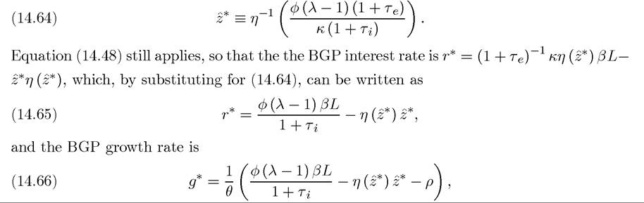
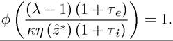
with z* given by (14.64). The following is now immediate:

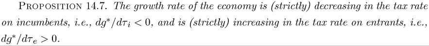
The result in this proposition is rather surprising and extreme. In Schumpeterian models, making entry more difficult, either with entry barriers or by taxing R&D by entrants, has negative effects on economic growth. Despite the Schumpeterian nature of the current model, here blocking entry increases equilibrium growth. Moreover, as Exercise 14.23 shows, in 534

the decentralized equilibrium of this economy there tends to be too much entry, so a tax on entry also tends to improve welfare. The intuition for this result is related to the main departure of this model from the standard Schumpeterian models. In contrast to the baseline Schumpeterian models, the engine of growth is still quality improvements, but these are undertaken both by incumbents and entrants. Entry barriers, by protecting incumbents, increase their value and greater value by incumbents encourages more R&D investments and faster productivity growth. Taxing entrants makes incumbents more profitable and this encourages further innovation by the incumbents. Taxes on entrants or entry barriers also further increase the contribution of incumbents to productivity growth.

Nevertheless, the result in this proposition should be interpreted with caution. The model in this section is special in that the R&D technology of incumbents is a linear. This linearity is important for the results in Proposition 14.7. Exercise 14.25 shows that the equilibrium can be characterized even when φ (z) is a concave function of z, and in this case, the effect of taxes on entrants is ambiguous, because it encourages R&D by incumbents and discourages R&D by entrants. Therefore, Proposition 14.7 should be read as emphasizing a particular new channel in the stark as possible way, not as a realistic description of how innovation will respond to tax policies.

14.3.5. Equilibrium Firm Size Distribution. The model presented in this section generates a dynamic equilibrium in which the economy, and thus the size of average firm, as measured by sales x (t), grows. To look at the firm size distribution, we therefore need to normalize firm sizes by the average size of firm, given by X (t), in (14.10). In particular, let

Let us continue to focus on equilibrium in which all incumbents exert the same R&D effort z*. In this case, since the unique equilibrium involves Xf (t) /X (t) = g* > 0, the law of motion for the normalized size of the leading firm in each industry can be written as

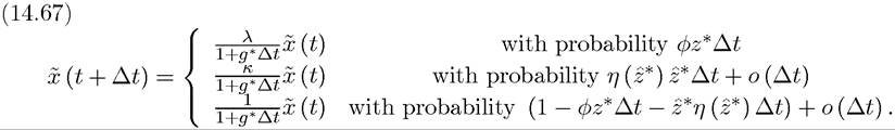
Notice that this expression does not refer to the growth rate of a single firm, but to the leading firm in a representative industry, and in particular, when there is entry, this leads to an increase in size rather than extinction.

1 — Γy^-χ). The Pareto distribution is attractive both because of its simplicity and tractability (see, for example, Section 15.8 in the next chapter), but also because the actual distribution of firm sizes in the US appears to fairly well approximated by a Pareto distribution with an exponent of one (e.g., Axtell, 2001). It is therefore a somewhat surprising and remarkable result that the simple model developed here, which was not designed to match the real-world firm size distributions, generates such a realistic distribution.

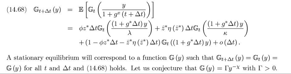
The following proposition shows that if a stationary distribution of (normalized) firm sizes exists, then it must take the form of the Pareto distribution with an exponent equal to 1. Recall that the Pareto distribution takes the form

Proposition 14.8. Let us focus on the equilibrium in which all incumbents choose R&D effort z*. Then, if a stationary distribution of (normalized) firm sizes exists, it is a Pareto distribution with exponent equal to 1, i.e.,

Proof. To prove this claim, let us suppose that a stationary distribution exists and consider an arbitrary time interval of ∆i > 0 and write

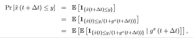
where 1{p} is the indicator function taking the value 1 if the statement P is correct and thus the first equation holds by definition. The second equation also holds by definition once g^x (t + ∆t) is designated as the (stochastic) growth rate of x between t and t + ∆t. Finally, the third equation follows from the Law of Iterated Expectations. Next, denoting 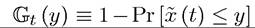as the complement of the cumulative density function, the previous equation yields

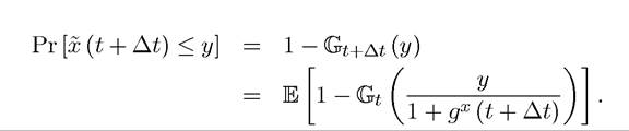
Therefore, we obtain the functional equation

536

Substituting this conjecture into the previous expression, we obtain

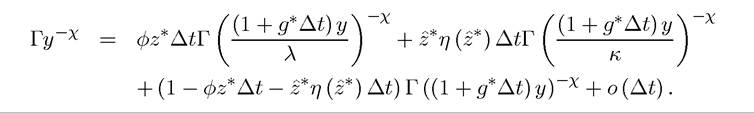
Rewriting this,

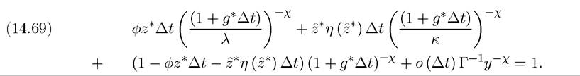
Now subtracting 1 from both sides, dividing by ∆t, and taking the limit as ∆t → 0, we obtain

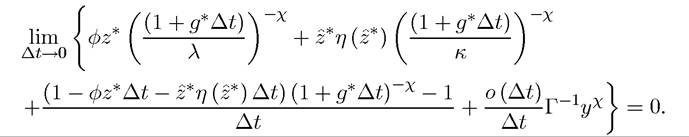
Taking the derivative of the penultimate term (which exists) and noting that 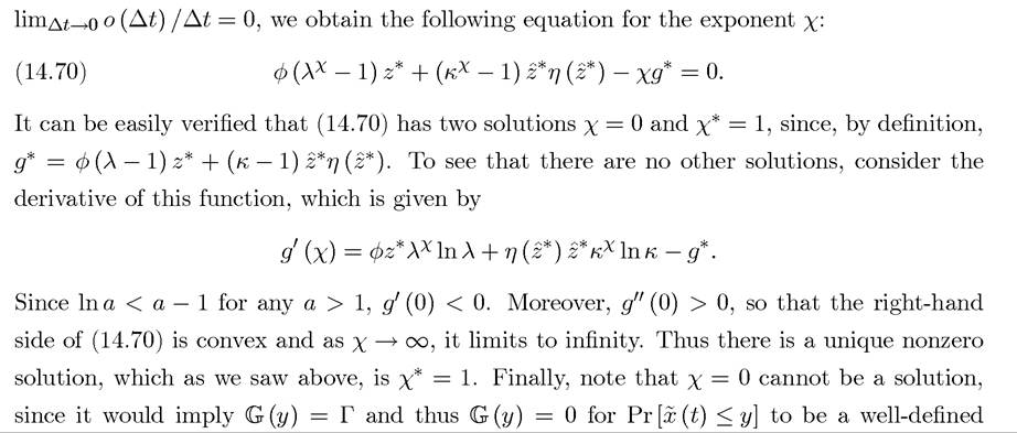distribution function. Yet this would imply that all firms have normalized size equal to zero, which violates the hypothesis that a stationary firm-size distribution exists. In contrast, which is a well-defined distribution function.

It can also be verified that no other function than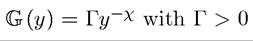can satisfy

this functional equation, completing the proof of the proposition. ?

In some ways, this result looks quite remarkable, since it generates a stationary firm-size distribution given by a Pareto distribution with an exponent of one, in a much simpler manner than any existing approaches, and does so despite the fact that the model was not designed to study firm size distributions. However, the proposition is proved under the hypothesis 537

that a stationary firm-size distribution exists. Unfortunately, the next corollary shows that this will not be the case.

Corollary 14.1. Let us focus on the equilibrium in which all incumbents choose R&D effort z*. Then a stationary firm-size distribution does not exist.

Proof. We know from Proposition 14.8 that if a stationary distribution exists, it must But the Pareto distribution is defined for all thus Γ should be the minimum normalized firm size. However, the law of motion of , (14.67), shows that it is possible for the normalized size of the firm (or of the relevant firm in an industry), x (t) to tend to zero. Therefore, Γ must be equal to 0, which implies that there does not exist a stationary firm-size distribution. ?

The essence of Corollary 14.1 is that with the random growth process in (14.67), the distribution of firm sizes will continuously expand. The “limiting distribution” will involve all firms being arbitrarily small relative to the average X (t) and a vanishingly small fraction of firms becomes arbitrarily large (so that average size X (t) remains large and continues to grow).

The result in Corollary 14.1 is closely linked to our focus on the equilibrium in which all incumbents choose the same R&D effort level. This focus is justified on theoretical grounds in Exercise 14.24. On empirical grounds, this assumption ensures that firm growth is inde­pendent of firm size, a regularity commonly referred to as Gibrat’s Law (e.g., Sutton, 1997). If z (ν, t | q) were a function of q, then firm growth would depend on firm size, violating Gibrat’s Law. Gibrat’s Law, despite its name, does not characterize the patterns of firm growth throughout the firm size distribution. In particular, the empirical evidence indicates that firm growth rates are indeed independent of firm size above a certain threshold, but are higher for small firms than for large firms (e.g., Hall, 1987). In light of this, consider the following candidate equilibrium. Let ε > 0 and suppose that

where

is relative quality in machine line ν at time t, andThis specification implies that

there is a slight deviation from Gibrat’s Law with firms below a certain relative size threshold growing faster than the rest (recall that average quality is proportional to average sales). Is straightforward to verify that there exists a BGP equilibrium in which incumbent R&D effort levels are given by (14.71) (see Exercise 14.25). Then we can prove the following result about the equilibrium firm-size distribution.

Proposition 14.9. Consider the BGP equilibrium in which incumbenteffort levels

are given by (14.71) forConsider the limiting case where

Then there exists a unique stationary firm-size distribution given by the Pareto distribution with an exponent of one.

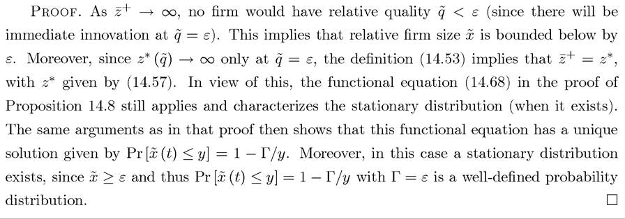
This proposition therefore shows that, if we focus on equilibria in which firms below a certain relative threshold have much higher innovation intensity, the equilibrium size distri­bution (in terms of normalized sizes) will be Pareto with an exponent equal to one.. This result is interesting and encouraging, since the distribution of firm sizes in the United States is very well approximated by the Zipf’s distribution (Axtell, 2001). Nevertheless, it should be noted that the approach adopted here is highly parsimonious (thus leaves out many relevant details) and the model takes a minimal departure from the baseline Schumpeterian model. Moreover, this model generates realistic firm-size distributions only when we select a par­ticular distribution of R&D levels among incumbents. A more detailed study of the issues related to firm dynamics and firm-size distributions requires more complex approaches that may capture richer dynamics, including more realistic models of entry and exit behavior of firms.

14.4.