Step-by-Step Innovations*

In the baseline Schumpeterian model and also in the extended Schumpeterian model of the previous section, new entrants could undertake innovation on any machine and did not need to have developed any knowhow on a particular line of business.

industries by stating that: “each of the major companies seems to have made more frequent contributions in a particular area,” and argues that this is because previous innovations in a field facilitate future innovations. This aspect is entirely missing from the baseline model of Schumpeterian growth, where any firm can engage in research to develop the next higher- quality machine (and in addition Arrow’s replacement effect implies that incumbents do not undertake R&D, though this aspect was relaxed and generalized in the previous section). A more realistic description of the research process may involve only a few firms engaging in continuous and cumulative innovation and competition in a particular product or machine line.

In this section, I will present a model of cumulative innovation of this type. Following Aghion, Harris, Howitt and Vickers (2001), we will refer to this as a model of step-by-step innovation. Such models are not only useful in providing a different conceptualization of the process of Schumpeterian growth, but they also enable us to endogenize the equilibrium market structure and allow a richer analysis of the effects of competition and intellectual property rights policy.

14.4.1. Preferences and Technology. Consider the following continuous time econ­omy with a unique final good. The economy is populated by a continuum of measure 1 of individuals, each with 1 unit of labor endowment, which they supply inelastically. To sim­plify the analysis, we assume that the instantaneous utility function takes a logarithmic form. Thus the representative household has preferences given by

where p > 0 is the discount rate and C (t) is consumption at date t.

Let Y (t) be the total production of the final good at time t. We assume that the economy is closed and the final good is used only for consumption (i.e., there is no investment or spending on machines), so that C (t) = Y (t).

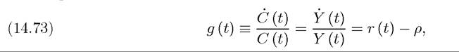
where this equation defines g (t) as the growth rate of consumption and thus output, and r (t) is the interest rate at date t.

The final good Y is produced using a continuum 1 of intermediate goods according to the Cobb-Douglas production function

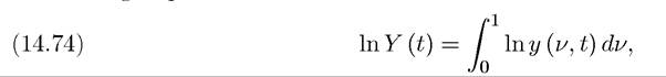
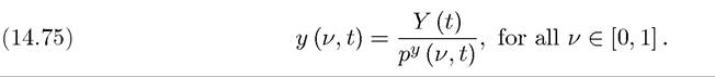
where y (ν,t) is the output of νth intermediate at time t. Throughout, we take the price of the final good (or the ideal price index of the intermediates) as the numeraire and denote the price of intermediate ν at time t by p^y (ν, t). We also assume that there is free entry into the final good sector. These assumptions, together with the Cobb-Douglas production function (14.74), imply that each final good producer will have the following demand for intermediates

Each intermediate ν ∈ [0,1] comes in two different varieties, each produced by one of two infinitely-lived firms. We assume that these two varieties are perfect substitutes and compete a la Bertrand. No other firm is able to produce in this industry. Firm i = 1 or 2 in industry ν has the following technology

where li (ν, t) is the employment level of the firm and qi (ν, t) is its level of technology at time t. The only difference between the two firms is their technology, which will be determined endogenously. As in the models studied so far, each consumer in the economy holds a balanced portfolio of the shares of all firms. Consequently, the objective function of each firm is to maximize expected profits.

The production function for intermediate goods, (14.76), implies that the marginal cost of producing intermediate ν for firm i at time t is

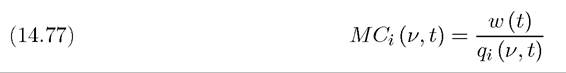
where w (t) is the wage rate in the economy at time t.

Let us denote the technological leader in each industry by i and the follower by —i, so that we have:

541

Bertrand competition between the two firms implies that all intermediates will be supplied by the leader at the limit price (see Exercise 14.27):

1828" class="lazyload" data-src="/files/uch_group77/uch_pgroup317/uch_uch7364/image/image1826.jpg">

Equation (14.75) then implies the following demand for intermediates:

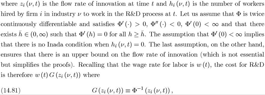
R&D by the leader or the follower stochastically leads to innovation. We assume that when the leader innovates, its technology improves by a factor λ > 1. The follower, on the other hand, can undertake R&D to catch up with the frontier technology. Let us assume that because this innovation is for the follower’s variant of the product and results from its own R&D efforts, it does not constitute infringement of the patent of the leader, and the follower does not have to make any payments to the technological leader in the industry.

R&D investments by the leader and the follower may have different costs and success probabilities. Nevertheless, we simplify the analysis by assuming that they have the same costs and the same probability of success. In particular, in all cases, we assume that each firm (in every industry) has access to the following R&D technology (innovation possibilities frontier):

and that the follower — i^,s technology at time t is

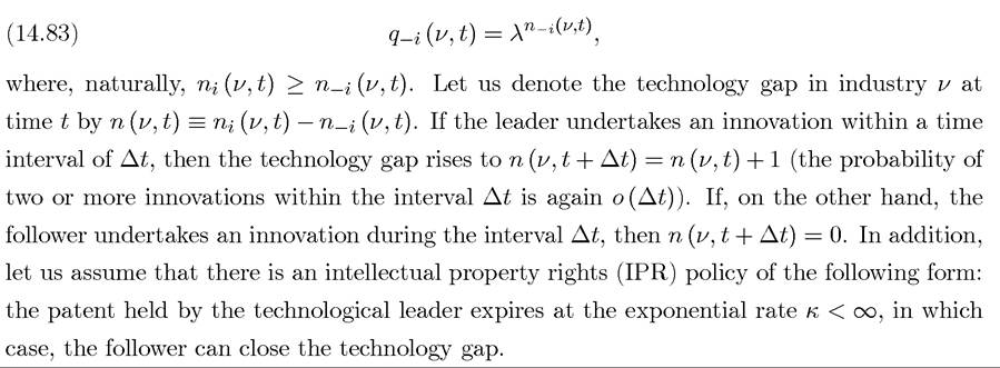
Given this specification, the law of motion of the technology gap in industry ν can be expressed as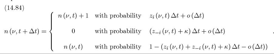

Here o (∆t) again represents second-order terms, in particular, the probabilities of more than one innovations within an interval of length ∆t.

We next write the instantaneous “operating” profits for the leader (i.e., the profits ex­clusive of R&D expenditures and license fees). Profits of leader i in industry ν at time t are

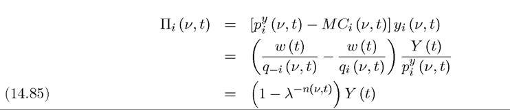
where recall that n (ν, t) is the technology gap in industry j at time t. The first line simply uses the definition of operating profits as price minus marginal cost times quantity sold. The second line uses the fact that the equilibrium limit price of firm i is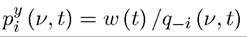

as given by (14.78), and the final equality uses the definitions of qi (ν,t) and q_-i (ν,t) from (14.82) and (14.83). The expression in (14.85) also implies that there will be zero profits in an industry that is neck-and-neck, i.e., in industries with n (j, t) = O. Followers also make zero profits, since they have no sales.

The Cobb-Douglas aggregate production function in (14.74) is responsible for the simple form of the profits (14.85), since it implies that profits only depend on the technology gap of the industry and aggregate output. This will simplify the analysis below by making the technology gap in each industry the only industry-specific payoff-relevant state variable.

The objective function of each firm is to maximize the net present discounted value of net profits (operating profits minus R&D expenditures and plus or minus patent fees).

output levels,the sequence of wages,the R&D decisions of all other

firms and policies as given. Note that as in the baseline model of Schumpeterian growth in Section 14.1, even though technology and output in each sector are stochastic, total output, Y (t), given by (14.74) is nonstochastic.

14.4.2. Equilibrium. Letdenote the distribution of industries over

different technology gaps, withFor example, μ₀ (t) denotes the fraction

of industries in which the firms are neck-and-neck at time t. Throughout, we focus on Markov Perfect Equilibria (MPE), where strategies are only functions of the payoff-relevant state variables. MPE is a natural equilibrium concept in this context, since it does not allow for implicit collusive agreements between the follower and the leader. While such collusive agreements may be likely when there are only two firms in the industry, in most industries there are many more firms and also many potential entrants, making collusion more difficult. Throughout, we assume that there are only two firms to keep the model tractable (see Appendix Chapter C for references and a further discussion of MPE). The focus on MPE allows us to drop the dependence on industry ν, thus we refer to R&D decisions by z_n for the technological leader that is n steps ahead and by z_-n for a follower that is n steps behind.

Given this, the equilibrium wage can be written as (see Exercise 14.28):

14.4.3. Steady-State Equilibrium. Let us now focus on steady-state (Markov Per­fect) equilibria, where the distribution of industriesis stationary, ω (t)

defined in (14.89) and g*, the growth rate of the economy, is constant over time (we refer to this as a steady-state Markov perfect equilibrium, since the potentially more accurate term “balanced growth path Markov perfect equilibrium” sounds awkward). We will estab­lish the existence of such an equilibrium and characterize a number of its properties. If the economy is in steady state at time t = 0, then by definition, we haveand

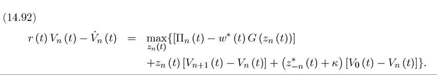
w (t) = wo exp (g*t). The two equations also imply that ω (t) = ω* for all t ≥ 0. Throughout, we assume that the parameters are such that the steady-state growth rate g^* is positive but not large enough to violate the transversality conditions. This implies that net present val­ues of each firm at all points in time will be finite and enable us to write the maximization problem of a leader that is n > 0 steps ahead recursively.

Standard arguments imply that the value function for a firm that is n steps ahead (or —n steps behind) is given by

In steady state, the net present value of a firm that is n steps ahead, V_n (t), will also grow at a constant rate g* for all n ∈ Z₊. Let us then define normalized values as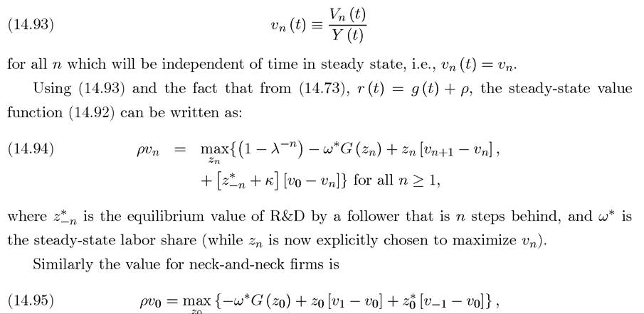

while the values for followers are given by

It is clear that these value functions and profit-maximizing R&D decision for followers should not depend on how many steps behind the leader they are, since a single innovation is sufficient to catch-up with the leader. Therefore, we can write

where v_-ι represents the value of any follower (irrespective of how many steps behind it is). The maximization problems involved in the value functions are straightforward and immediately yield the following profit-maximizing R&D decisions

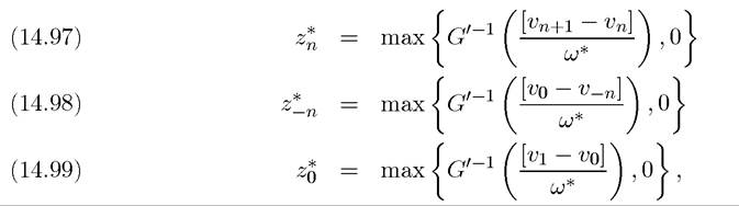
where G^0-1 (∙) is the inverse of the derivative of the G function, and since G is twice con­tinuously differentiable and strictly concave,is continuously differentiable and strictly increasing. These equations therefore imply that innovation rates, theare increasing in the incremental value of moving to the next step and decreasing in the cost of R&D, as measured by the normalized wage rate, ω*. Note also that since G⁰ (0) > 0, these R&D levels can be equal to zero, which is taken care of by the max operator.

The response of innovation rates,to the increments in values,is the key

economic force in this model. For example, a policy that reduces the patent protection of leaders that are n + 1 steps ahead (by increasing κ) will make being n + 1 steps ahead less profitable, thus reduce v_n+ι — v_n andThis corresponds to the standard disincentive effect of relaxing IPR protection. However, relaxing IPR protection may also create a beneficial composition effect; this is because, typically,is a decreasing sequence, which

implies thatis higher than(see Proposition 14.13 below). Weaker patent

protection (in the form of shorter patent lengths) will shift more industries into the neck- and-neck state and potentially increase the equilibrium level of R&D in the economy.

Given the equilibrium R&D decisions, the steady-state distribution of industries across states μ* has to satisfy the following accounting identities: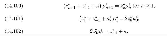

The first expression equates exit from state n + 1 (which takes the form of the leader going one more step ahead or the follower catching-up the leader) to entry into this state (which takes the form of a leader from the state n making one more innovation). The second equation, (14.101), performs the same accounting for state 1, taking into account that entry into this state comes from innovation by either of the two firms that are competing neck-and-neck. Finally, equation (14.102) equates exit from state 0 with entry into this state, which comes from innovation by a follower in any industry with n ≥ 1.

The labor market clearing condition in steady state can then be written as

with complementary slackness.

The next proposition characterizes the steady-state growth rate in this economy:

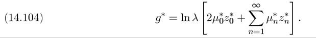
Proposition 14.10. The steady-state growth rate is given by

Proof. Equations (14.89) and (14.91) imply

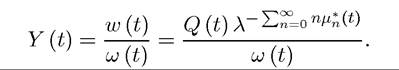
Since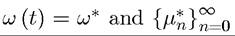are constant in steady state, Y (t) grows at the same rate as

Q (t). Therefore,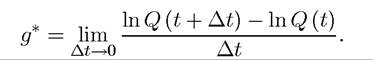

During an interval of length ∆t, we have that in the fractionof the industries with

technology gap n ≥ 1 the leaders innovate at a rateand in the fraction μθ of

the industries with technology gap of n = 0, both firms innovate, so that the total innovation rate is :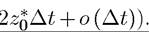Since each innovation increases productivity by a factor λ, we obtain

the preceding equation. Combining these observations, we have

Subtracting lnQ (t), dividing by ∆t and taking the limit as ∆t → 0 gives (14.104). ?

This proposition clarifies that the steady-state growth comes from two sources:

(1) R&D decisions of leaders or of firms in neck-and-neck industries.

(2) The distribution of industries across different technology gaps,

The latter channel reflects the composition effect discussed above. This type of compo­sition effect implies that the relationship between competition and growth (or intellectual property rights protection and growth) is more complex than in the models we have seen so 548

far, because such policies will change the equilibrium market structure (i.e., the composition of industries).

Definition 14.1. A steady-state equilibrium is given by {μ*, v, z*, ω*, g*) such

We next provide a characterization of the steady-state equilibrium. The first result is a technical one that is necessary for this characterization.

Sincethis impliescontradicting the hypothesis that, and

establishing the desired result,

Consequently,is nondecreasing andis (strictly) increasing. Since a

nondecreasing sequence in a compact set must converge,id="Picutre 1880" class="lazyload" data-src="/files/uch_group77/uch_pgroup317/uch_uch7364/image/image1878.jpg">converges to its limit

point, v∞, which must be strictly positive, sinceis strictly increasing and has a nonnegative initial value. This completes the proof. ?

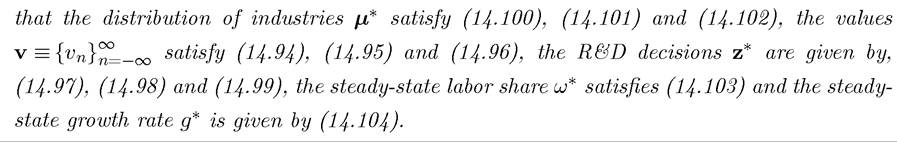
A potential difficulty in the analysis of the current model is that we have to determine R&D levels and values for an infinite number of firms, since the technology gap between the leader and the follower can, in principle, take any value. However, the next result shows that we can restrict attention to a finite sequence of values:

Proposition 14.12. There exists n* ≥ 1 such that

Proof. See Exercise 14.29. ?

The next proposition provides the most important economic insights of this model and shows thatis a decreasing sequence, which implies that technological lead­

ers that are further ahead undertake less R&D. Intuitively, the benefits of further R&D investments are decreasing in the technology gap, since greater values of the technology gap translate into smaller increases in the equilibrium markup (recall (14.85)). The fact that leaders that are sufficiently ahead of their competitors undertake little R&D is the main reason why composition effects play an important role in this model. For example, all else equal, closing the technology gap across a range of industries will increase R&D spending and equilibrium growth (though, as discussed in the previous section, this may not always increase welfare, especially if there is a strong business stealing effect).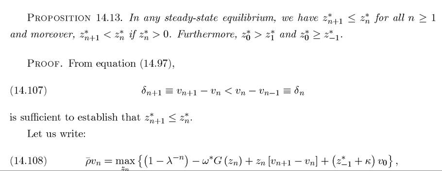

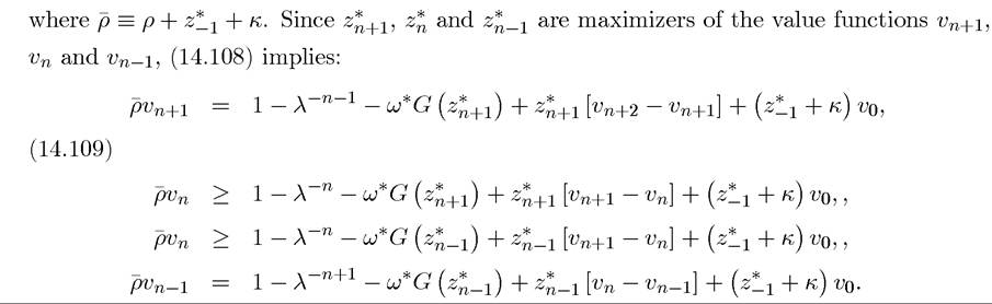
Now taking differences with ρv_n and using the definition of δ_n's, we obtain

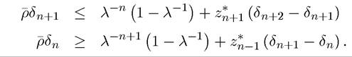
Therefore,

This proposition therefore shows that the highest amount of R&D is undertaken in neck- and-neck industries. This explains why composition effects can increase aggregate innovation.

551

Exercise 14.31 shows how a relaxation of intellectual property rights protection can increase the growth rate in the economy.

So far, we have not provided a closed-form solution for the growth rate in this economy. It turns out that this is generally not possible, because of the endogenous market structure in these types of models. Nevertheless, it can be proved that a steady state equilibrium exists in this economy, though the proof is somewhat more involved and does not generate additional insights for our purposes (see Acemoglu and Akcigit, 2006).

An important feature of this model is that equilibrium markups are endogenous and evolve over time as a function of competition between the firms producing in the same product line. More importantly, when a particular firm is sufficiently ahead of its rival, it undertakes less R&D. Therefore, this model, contrary to the baseline Schumpeterian model and also contrary to all expanding varieties models, implies that greater competition may lead to higher growth rates. Greater competition generated by closing the gap between the followers and leaders induces the leaders to undertake more R&D in order to escape the competition from the followers.

14.5.